| Physics 728 |
Radio Astronomy: Lecture #1
|
Prof. Dale E. Gary
NJIT
|
Introduction to Radio Astronomy
Overview of Radio Emission
from Astronomical Objects
The Radio Sky
When we look at
the sky at night with our unaided eyes, we see about 2000 stars of various
levels of brightness, and if we are far from city lights we may see the
faint band of the Milky Way, which is the light from billions of stars
making up our galaxy. But if our eyes were able to see radiowaves,
the sky might look like the image below.
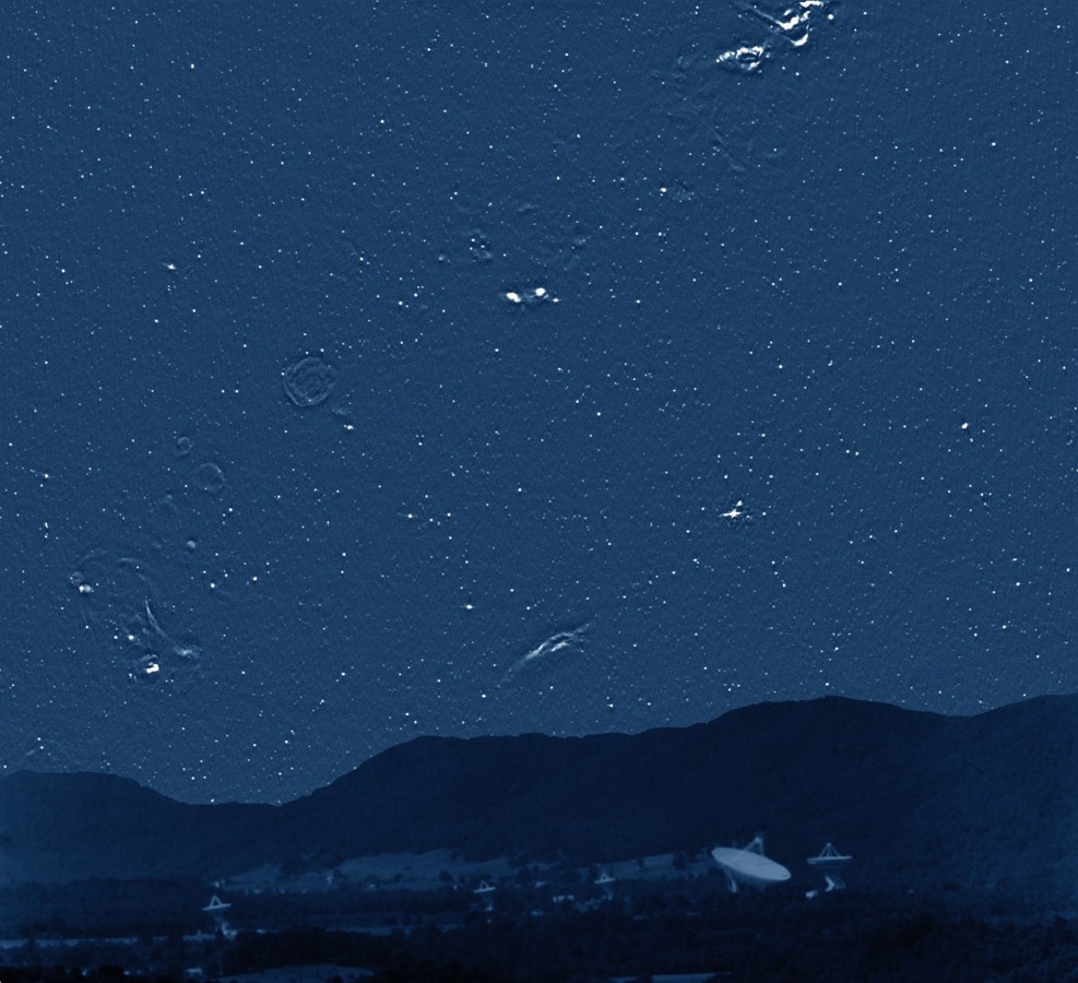
(c) National Radio Astronomy
Observatory / Associated Universities, Inc. / National Science Foundation
It may appear similar to
the starry sky, but in fact most of the point-like objects are not stars,
but luminous radio galaxies billions of light years away. The larger
sources are ionized clouds of hydrogen, or supernova remnants.
Looking toward the center
of our galaxy, our radio eyes would see a large variety of strange features,
most of which are not visible in other wavelengths.
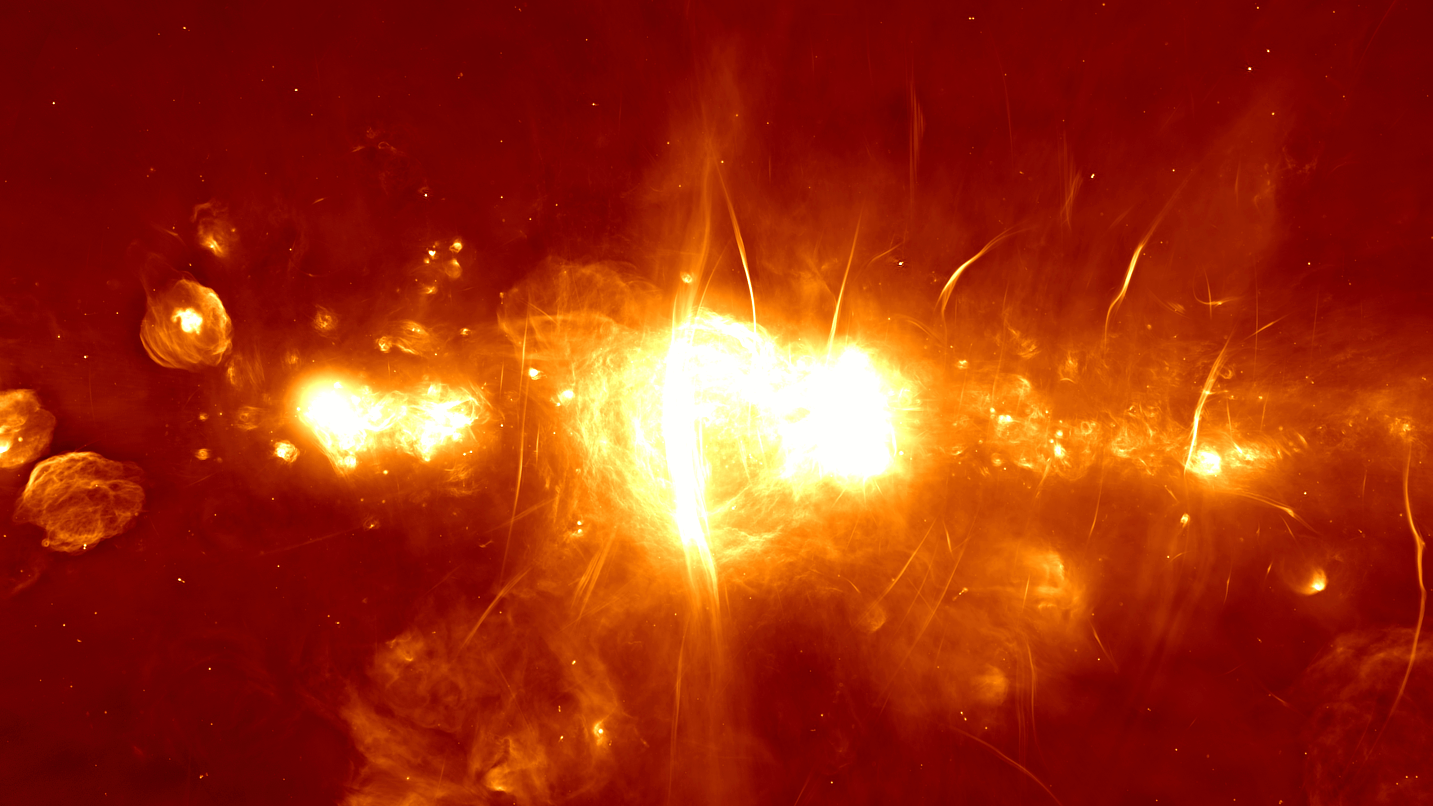
The Galactic Center - First Light from MeerKAT Radio Telescope
Credit: https://www.gizmodo.com.au/2018/07/new-south-african-telescope-releases-epic-image-of-the-galactic-centre/
Owens Valley Long Wavelength Array Movie
The Electromagnetic Spectrum
You should all be
aware of the different types of radiation that make up the electromagnetic
spectrum, but it is worthwhile to list the names of the different types
of emission, in energy, or frequency) order:
-
gamma rays (> ~1 MeV)
-
hard X-rays (10-1000 keV)
-
soft X-rays (1-10 A)
-
EUV (~100 A)
-
UV (~1000 A)
-
visible (4000-7000 A -- 400-700
nm)
-
near IR (~1 micron)
-
IR (10 microns)
-
THz (~100 microns--3000 GHz)
-
submillimeter (300 GHz - 700
GHz)
-
millimeter (30 GHz - 300 GHz)
-
microwave (3 GHz - 30 GHz)
-
decimeter (300 MHz - 3 GHz)
("cable" TV/UHF band)
-
meterwave (30 MHz - 300 MHz)
(TV/FM/HF band)
-
dekameter (3 MHz - 30 MHz) (Shortwave
-
AM band (0.5 MHz - 1.7 MHz)
etc.
|
 |
Note that the units change
as we go from top to bottom--use energy units near the top, then switch
to wavelength units, then switch to frequency units. This is purely
a matter of convenience and convention. We could stick with energy,
or wavelength, or frequency throughout, but the range of 6 or 7 decades
makes it inconvenient to stick with one measure. The relationships
among energy, frequency, and wavelength are, of course:
E = hn =
hc/l.
For the purposes of this course,
we will be concentrating on techniques of interferometry and synthesis
imaging that work for the range from submillimeter to dekameter, although
there are practical difficulties at both extremes, and it is currently
most common to use interferometry in the millimeter to meterwave range.
There are on-going efforts to extend interferometry to both higher frequencies
(submillimeter--ALMA) and lower frequencies (space arrays).
Why Observe At Radio Wavelengths?
There are many reasons
why it is advantageous to observe at radio wavelengths.
Advantages of Radio
-
Radio waves reach the ground
-
Can observe objects or phenomena
that are difficult or impossible to detect in other wavelength ranges
-
Can use radio emission for quantatitive
physical diagnostics of object parameters
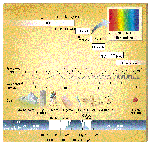
The first reason is simply that
it is possible to observe radio waves from the ground. As shown in
the figure below, spacecraft are needed to observe astronomical objects
in gamma rays, X-rays, UV, and IR, while ground observations are possible
in the visible, some parts of the near IR, and the radio. NJIT has
solar observatories exploiting all of these ground windows.
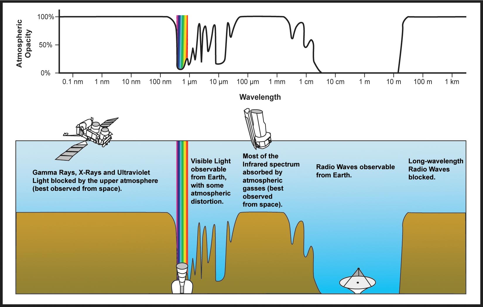
Credit: NASA/IPAC
Note that the window
closes at the long-wavelength end of the spectrum--not because of the atmosphere,
which remains transparent to long-wavelength radio waves--but rather due
to the ionosphere, which reflects the radiation.
A second reason is that some
objects and phenomena are invisible or hard to detect in other wavelengths,
and can only be seen, or can be seen with greater sensitivity, in the radio.
Here are a few of many many examples from which we could choose:
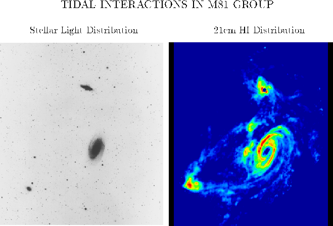
Neutral hydrogen traces
interactions among galaxies in the M81 group.
(c) National Radio Astronomy
Observatory / Associated Universities, Inc. / National Science Foundation
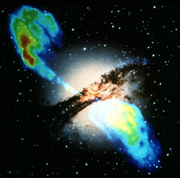
Centaurus A -- peculiar
galaxy with radio lobes. From HST
web site.
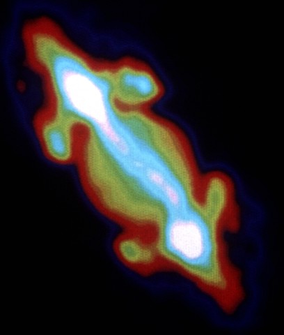
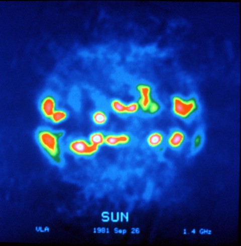
Jupiter's Radiation Belt
The Sun
.
(c) National Radio Astronomy
Observatory / Associated Universities, Inc. / National Science Foundation
The third important reason
to explore astronomical objects in radio wavelengths is that the emission
properties provide quantitative physical information about conditions in
the source. We will see that radio emission is produced in a large
number of ways. The low-energy radio photons are relatively easy
to produce, which makes radio emission sensitive to a great many parameters.
However, the number of mechanisms is itself a problem. Before one
can use the emission to give information, one must first determine which
radio emission mechanism is responsible for the emission. In
practice, the most accurate way to determine the emission mechanism is
to have spectral information,
since different emission mechanisms have different characteristic spectral
properties. In addition to helping to determine the emission mechanism,
quantifying spectral properties such as peak brightness, peak frequency,
spectral slopes, etc., also provides quantitative diagnostic parameters.
For all of these reasons
and more, the radio range of wavelengths is as essential as gamma ray,
X-ray, UV, optical, and IR for providing a complete picture of the physical
nature of astronomical sources.
Overview of Radio Instrumentation
What Is Different About Radio
Instrumentation?
Astronomical telescopes
that work in the radio range look and operate very differently from the
more familiar optical instrumentation. In fact, the "radio" range
is so broad (6 or 7 orders of magnitude) that instruments at the low end
of the frequency range look very different from those at the high end.
We will take a brief look at the differences, using some existing or planned
telescopes as examples.
Single Element Instruments
The term "single
element" means either single parabolic dishes, or in some cases single
dipole elements. Here are a few pictures:
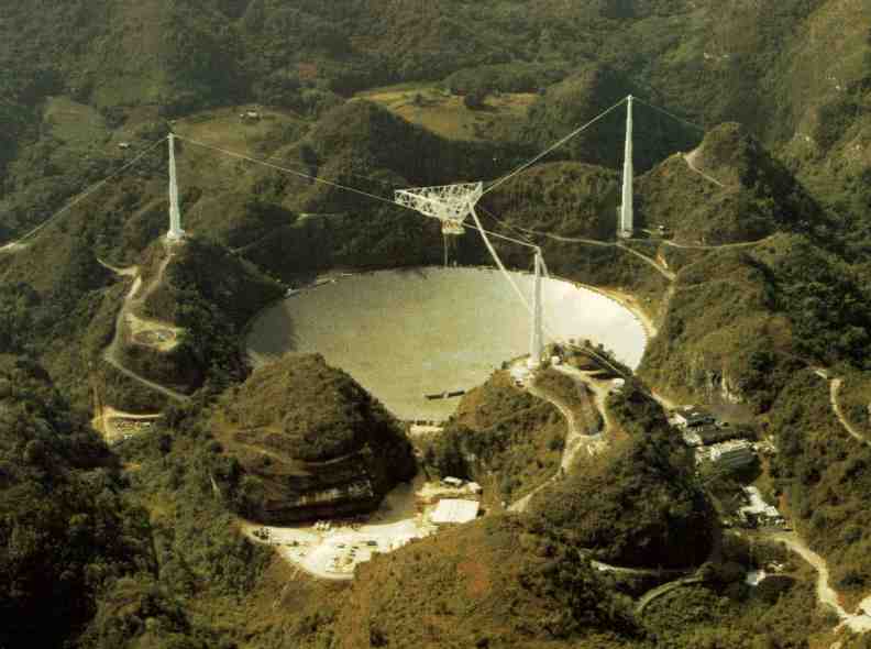
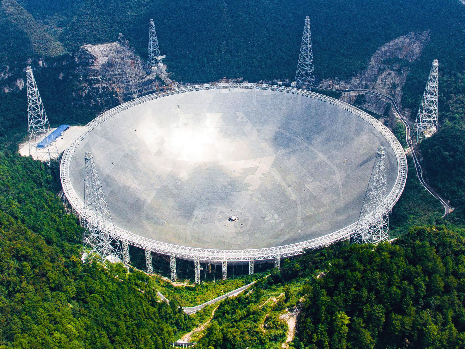
Arecibo: The largest single
dish in the world, 306 m
(c) Cornell University /
National Science Foundation
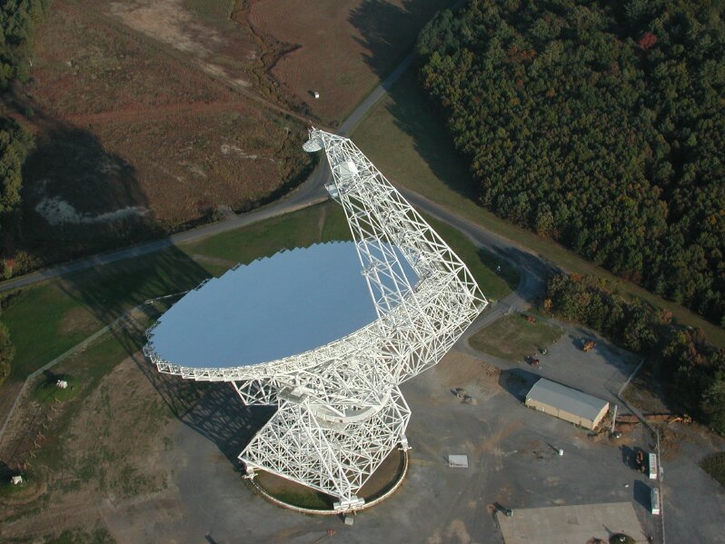
Green Bank Telescope (GBT):
The largest fully steerable single dish in the world, 100 x 110 m
(c) National Radio Astronomy
Observatory / Associated Universities, Inc. / National Science Foundation
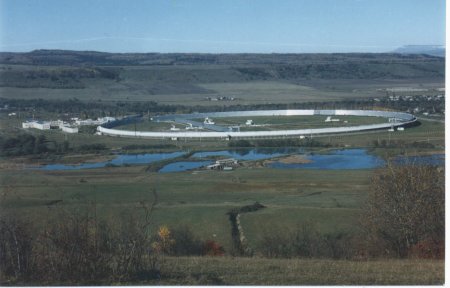
RATAN 600: Diameter 600
m, part of a "dish" reflecting surface
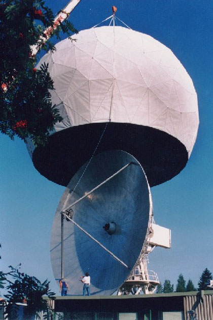
Metsahovi: Large mm dish
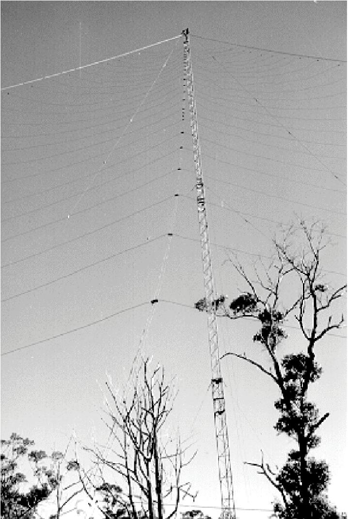
Bruny Island Radio Spectrograph
Single radio elements
have limited spatial resolution (the diffraction limit of the telescope).
This diffraction limited resolution is proportional to wavelength (as it
is also for optical telescopes, but it seems more extreme for radio telescopes
due to the huge range of wavelengths over which they are typically used).
The diffraction limit for a circular aperture of diameter D
is q ~ 1.22 l/D,
where q
is the angular diameter of the Airy Disk at the half-power point (the full-width-half-maximum,
or FWHM) in radians. At a frequency of 5 GHz, even the Arecibo dish
has an angular resolution of only about 50 arcseconds. The fully-steerable
GBT has a resolution at this frequency of only 150 arcseconds.
Because of the limited spatial
resolution of single element telescopes, sophisticated techniques have
been developed to combine single elements into multiple-element arrays,
which work together to form a single telescope. In such arrays, the
spatial resolution is determined not by the size of the individual elements,
but rather by the maximum separation between elements, which is referred
to as the baseline length, B.
With an interferometer, the diffraction limit is q
~ l/B, where
B
can extend to many (even thousands of) km.
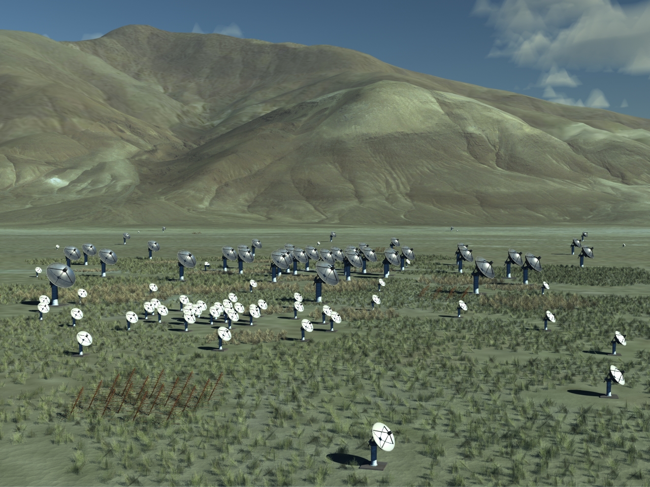
Interferometers
We now show some
examples of interferometer arrays:
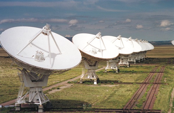
Close-up of VLA (Very Large
Array)
(c) National Radio Astronomy
Observatory / Associated Universities, Inc. / National Science Foundation
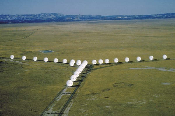
Aerial view of VLA in its
most compact configuration.
(c) National Radio Astronomy
Observatory / Associated Universities, Inc. / National Science Foundation
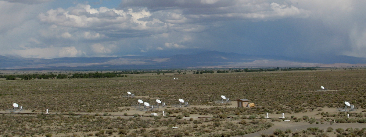
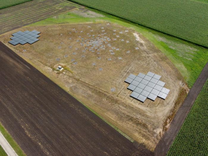
Ten antennas of NJIT's 13-antenna Expanded Owens Valley Solar Array
(EOVSA)
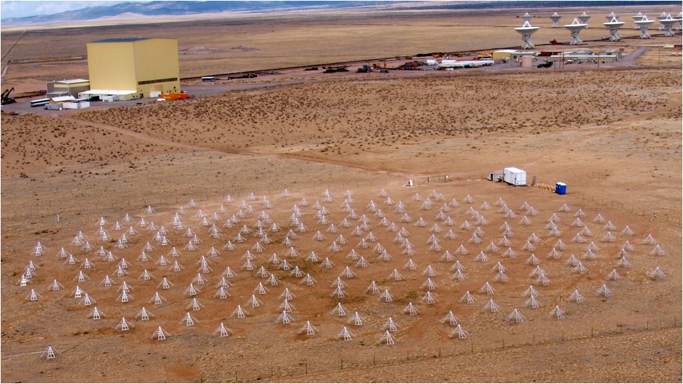
The Long Wavelength Array (LWA) station at the VLA in New Mexico (See LWA-TV) (Univ. of New Mexico)
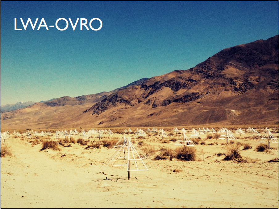
The Long Wavelength Array (LWA) station at Owens Valley in California (Gregg Hallinan, Caltech)
North arm of the Nancay
Radioheliograph (Meudon, Observatoire de Paris)
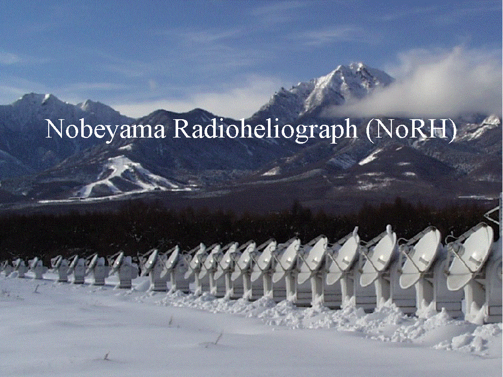
Nobeyama Radioheliograph
(National Astronomical Observatory of Japan)
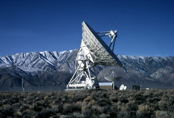
One of 10 antennas of the
Very Long Baseline Array (VLBA) -- this one at OVRO.
(c) National Radio Astronomy
Observatory / Associated Universities, Inc. / National Science Foundation

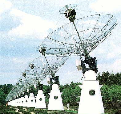
Site locations for the entire
10-station VLBA
(c) National Radio Astronomy
Observatory / Associated Universities, Inc. / National Science Foundation
-
Low Frequency Array (LOFAR)
-
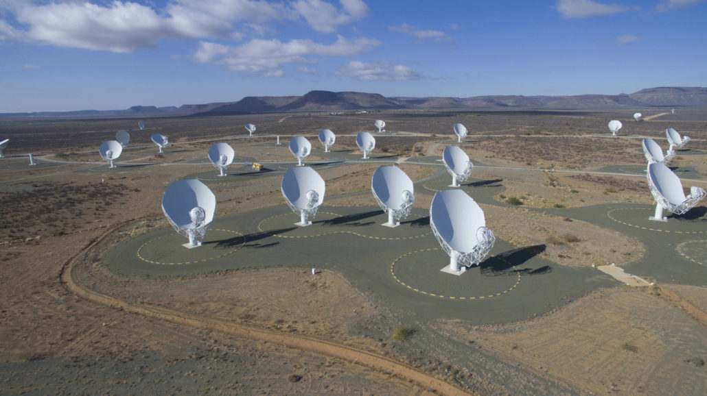
Atacama Large Millimeter Array
(ALMA)
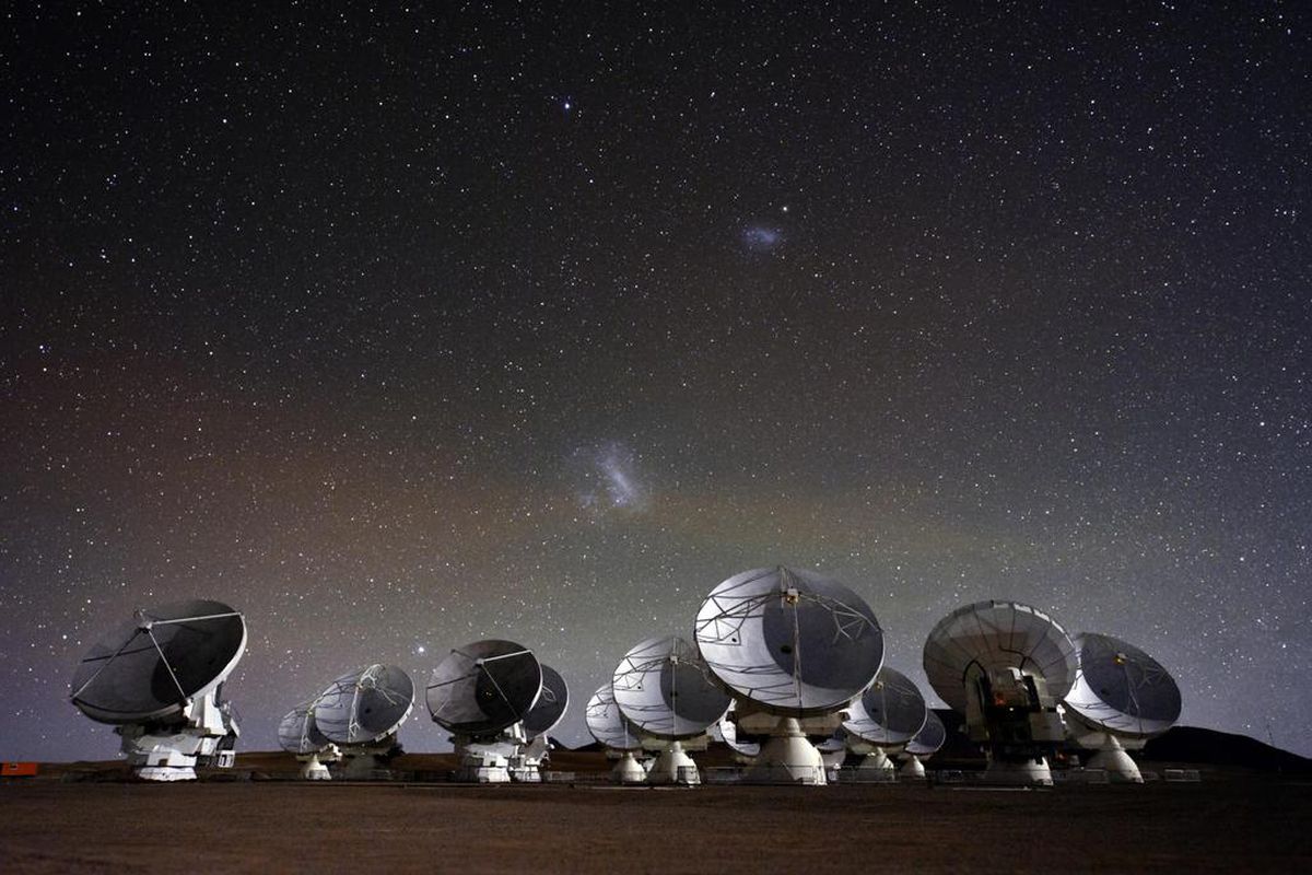
Atacama Large Millimeter Array (ALMA)
(c)
ALMA (ESO/NAOJ/NRAO)
Future arrays, now under
consideration/construction:
- Frequency Agile Solar Radiotelescope
(FASR)
Brightness Temperature
and Flux Density
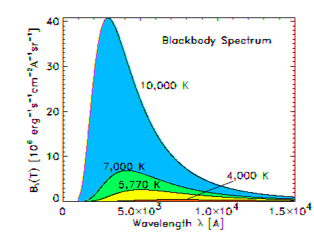
Planck Function
You should all be
familiar with the basics of black-body radiation. By simply observing
how hot objects behave, 19th century scientists came up with the following
empirical laws.
-
the peak wavelength shifts proportional
to temperature lmaxT
= 2.898x10⁻³
m K. (Wien Displacement Law)
-
the intensity increases as the
square of the frequency at low frequencies (Rayleigh-Jeans Law)
-
the intensity decreases exponentially
at high frequencies (Wien Law)
-
the flux of radiation emitted
by a blackbody increases as the fourth-power of the temperature (Stefan-Boltzmann
Law)
A plot of this behavior for
several temperatures as a function of wavelength is shown in the figure
below.
 The functional form that corresponds
to these curves is called the Planck function,
which was derived by Max Planck by introducing the Planck constant h
= 6.63 x 10⁻³⁴ J s,
and postulating that photon energies were quantized in units of hn.
This was the beginning of the quantum theory, which was later extended
to matter as well as radiation. This function has two forms, written
below, which are related by Bl(T)
dl
= Bn(T)
dn.
The functional form that corresponds
to these curves is called the Planck function,
which was derived by Max Planck by introducing the Planck constant h
= 6.63 x 10⁻³⁴ J s,
and postulating that photon energies were quantized in units of hn.
This was the beginning of the quantum theory, which was later extended
to matter as well as radiation. This function has two forms, written
below, which are related by Bl(T)
dl
= Bn(T)
dn.
| |
|
2hc2/l5
|
|
| Bl(T) |
= |
|
(wavelength form)
(1) |
| |
|
ehc/lkT
- 1 |
|
| |
|
2hn3/c2
|
|
| Bn(T) |
= |
|
(frequency
form) (2) |
| |
|
ehn/kT
- 1 |
|
-
To derive the Wien displacement
law, find the maximum of the function by setting dBl(T)
/ dl = 0,
to get lmaxT
= hc/5k = 2.898 x 10⁻³
m
-
To derive the Rayleigh-Jeans
law, expand ehn/kT
in Bn(T)
for
hn
<< kT to get Bn(T)
= 2kTn2/c2
-
To derive the Wien Law, expand
ehn/kT
in Bn(T)
for
hn
>> kT to get Bn(T)
= (2hn3/c2)e-hn/kT
-
To derive the Stefan-Boltzmann
Law, integrate Bl(T)
over
all wavelengths--hint: use the relation
 |
inf |
u3du
|
|
p4 |
|
|
= |
|
| 0 |
eu-
1 |
|
15 |
--to get the flux
F
= sT4,
where s= 2p5k4/(15c2h3)
= 5.669 x 10⁻⁸
W/m2/K4
is the Stefan-Boltzmann constant.
Rayleigh-Jeans Limit
The Rayleigh-Jeans
limit is the Planck function in the limit of low-energy photons, hn
<< kT, which we argue is the
relevant limit for any source that produces radio emission. To see
this, take a relatively high radio frequency, say 100 GHz, and ask how
cool the source must be in order that the above condition be violated (i.e.
for hn ~ kT).
We have
T = hn/k
= (6.63 x 10⁻³⁴
J s)(1 x 10¹¹ s-1)/1.38
x 10-23
J/K = 4.8 K !
So even very cold sources at
high frequencies still meet the Rayleigh-Jeans criterion. This turns
out to be especially useful for radio astronomy, which we will discuss
in a moment. But first, let's look at another plot of the Planck
function, with axes suitable for a visual appreciation of the Rayleigh-Jeans
limit.
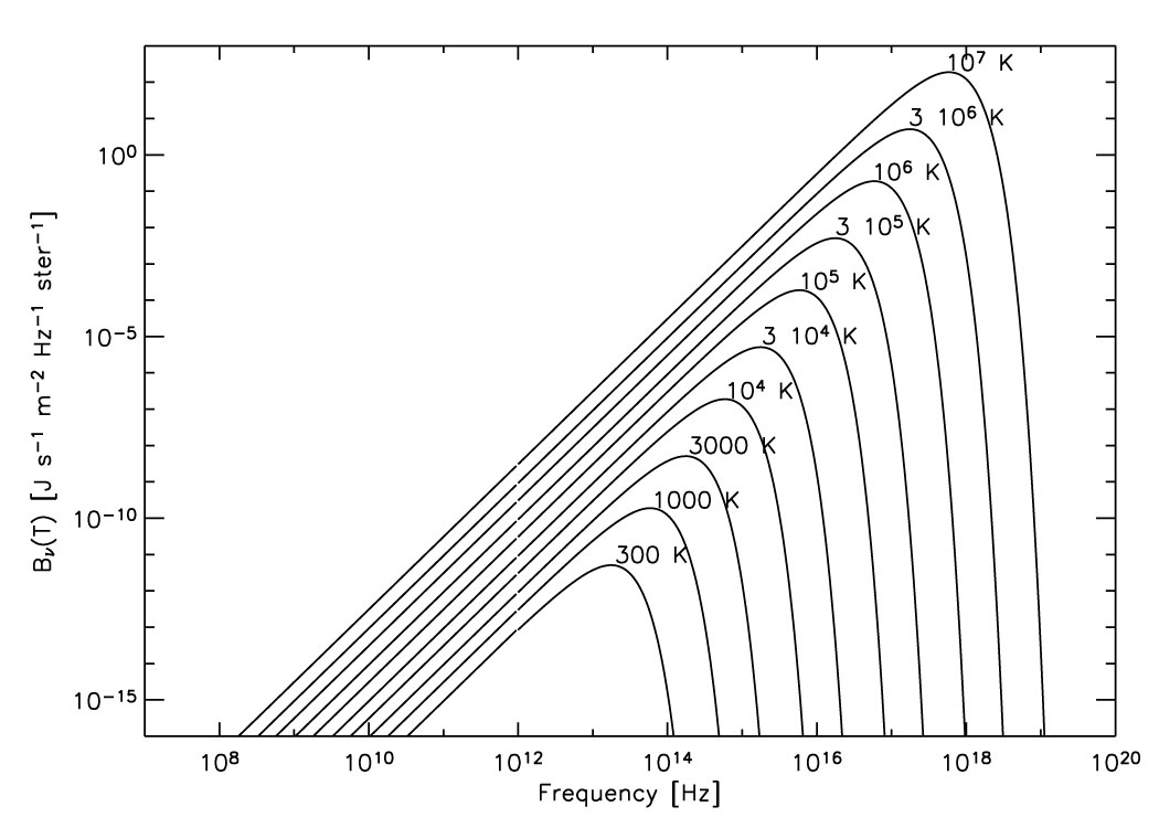
By plotting Bn(T)
on a log-log plot, the part of the curve that obeys the Rayleigh-Jeans
Law,
Bn(T)
= 2kTn2/c2
(3),
is very obvious--it is the straight
line portion with a slope of 2. Here you can see that changing the
temperature over many orders of magnitude just increases the intensity
linearly, and that it is valid over the entire range of radio frequencies
all the way to THz (1012 Hz).
Surface Brightness (Intensity)
and Flux Density
The monochromatic
intensity I(n)
has units of J m-2
s-1 Hz-1
sr-1, where sr = sterradians
is the unit of solid angle,
DW.
By comparing these units with the Planck function, we see that they are
the same. The Planck function gives the monochromatic intensity of
the blackbody that it represents. The intensity,
or surface brightness, is then
integrated over all frequencies:
| I |
= |
|
I(n)dn
(units:
J m-2
s-1 sr-1). |
Integrate this again
over angular area to get the flux F:
| F |
= |
|
I dW
(units: J m-2
s-1, or W m-2) |
which is just the
power per unit area. In radio astronomy, we often discuss a related
quantity called the flux density,
which is the monochromatic intensity (or the Planck function) integrated
over solid angle:
| S |
= |
|
I(n) dW
(units: W m-2
Hz-1)
(4) |
In fact, the flux density
is a fundamental quantity measured by radio telescopes, and is the basis
for two different units:
1 Jansky (Jy) =
10-26 W m-2
Hz-1
1 Solar Flux Unit (sfu)
= 10-22 W m-2
Hz-1 = 10000 Jy.
The quantity that a radio telescope
measures is the flux density over some band Dn,
so the strength of radio sources in the sky are often specified in Jy.
Likewise, the strength of solar sources, especially solar radio bursts,
are often specified in sfu.
Brightness Temperature
We are now ready
to show a great conceptual simplification that the Rayleigh-Jeans limit
gives to the discipline of radio astronomy. We have so far been talking
about blackbodies, which are by definition optically thick and in thermal
equilibrium. What if a source is not optically thick? In that
case, its emission will appear weaker (lower intensity) than if it were
optically thick. Whether or not a source is optically thick is a
function of frequency. As it turns out, many radio-emitting plasmas
are optically thick at low frequencies, but optically thin at high frequencies.
In this case, the brightness follows the Planck function up to some frequency,
then begins to fall away as it becomes more and more optically thin with
frequency. Schematically, it looks something like this:
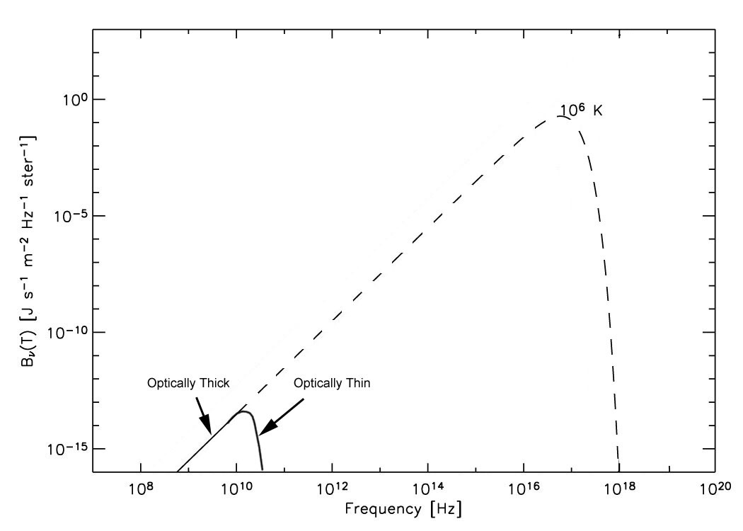
Radio spectrum for a 106
K plasma that is optically thick below about 10 GHz, and optically thin
at higher frequencies.
The brightness below 10 GHz corresponds to a million degree blackbody.
We will discuss optical depth
in more detail in two weeks, when we discuss radiative transfer.
For now, we just want to develop the idea of brightness
temperature.
In the Rayleigh-Jeans limit,
a blackbody has a temperature given by the Rayleigh-Jeans Law, eq (3),
i.e.
T = Bn(T)c2/2kn2
so as long as the plasma in
the above figure is optically thick, we can use the brightness of the emission
to determine the plasma temperature. But when it is optically thin,
the brightness, or intensity, is less than the Planck function. Nevertheless,
we can still talk about a brightness temperature, or the equivalent temperature
that a blackbody would have in order to be as bright. The brightness
temperature is the same as the true temperature only for an optically thick
blackbody. We designate the brightness temperature as Tb.
Using this notation, the flux density measured by a radio telescope becomes:
| S |
= |
|
2kTbn2/c2
dW |
= 2kn2/c2 |
|
Tb dW
(5) |
where we have substituted
Bn
for I(n)
in (4), and used (3). So the flux density measured by a radio telescope
is just the brightness temperature integrated over the source, times some
fundamental constants and frequency-squared.
So far, eq (5) pertains only
to thermal emission, but we can extend it to all radio emission simply
by considering non-thermal sources as having an effective
temperature Teff.
For a single electron of energy E,
its effective temperature is just its kinetic temperature Teff
= E/k.
To summarize, then, the brightness
temperature is the equivalent temperature a black body would have in order
to be as bright as the observed brightness. It is important to realize
that this is a useful concept only for radiation that obeys the Rayleigh-Jeans
Law.
One last point to make is
the limit of the integral in eq (5). We earlier mentioned the resolution
of a single dish antenna of diameter D,
as q ~ 1.22 l/D.
This is also the width of the field of view of the antenna--only a source
in an area of the sky within this angular distance can be seen. The
field of view is also called the beam.
Let's look at some consequences of this.
-
Unresolved (point) Source: If
the antenna is pointing at a source with a very small size, the flux density
that it measures is the brightness integrated over the entire source, i.e.
the total flux density of the source. In this case, the integral
(5) is to be taken over the source.
-
Extended Source: If the antenna
is pointing at an extended source, part of which falls outside the field
of view, it will measure only the flux from the source within the beam.
In this case, the integral (5) is to be taken over the beam size.