Interferometer Response to Plane Waves

The basic unit of an interferometer array is the single baseline between two antennas, as shown in Figure 1, below.  A plane wave incident from directly overhead will arrive at the antennas in phase, and if the signal travels the same distance through cables to the correlator (shown with an X in the figure, because it is just a multiplication), the signal from the two antennas will give a maximum response.

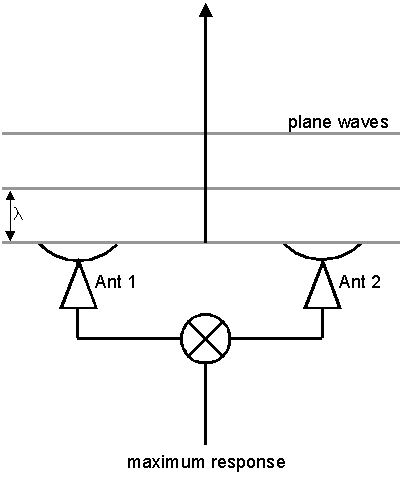
Figure 1: Geometry of an interferometer baseline, with plane
waves incident vertically, of wavelength l.

If the plane wave comes from a slightly different direction, it will arrive at the antennas slightly out of phase, and the response will be less, except that when the waves arise exactly 1 wavelength out of phase the response will again be a maximum, as shown in Figure 2.

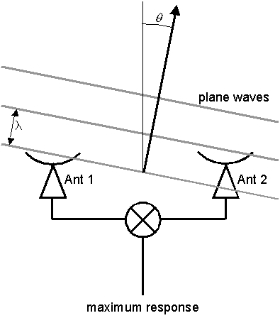
Figure 2: The same baseline as in FIgure 1, but for waves incident from
an angle q  from the vertical.  The waves arrive at the antennas again
exactly in phase, because the angle is such that the difference in path length is l.

The angle for which the secondary maximum occurs is

q = sin^-1l/B                                               (1)

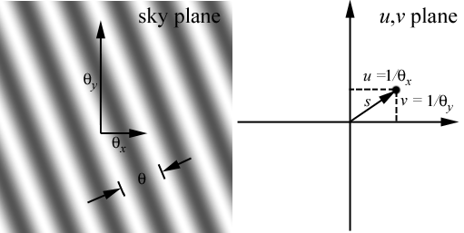
where B is the baseline length, or distance between antennas.  The angle q  is also called the fringe spacing, as introduced in Lecture 4.  Additional maxima occur at integer multiples of q, to provide the fringe pattern across the sky.  Recall from Lecture 4 that in two dimensions the fringe pattern looks like the left panel of the figure below.

If we have a truly monochromatic system, the fringes will extend all the way across the sky with the same amplitude.  However, in practice our observation will be done over some bandwidth Dn.  Since the spacing between fringes depends on wavelength, frequencies in one part of the band will have fringes with one spacing, and fringes in another part of the band will have another spacing, so that at large angles the frequencies start interfering with each other.  At what value of q will there be an extra pathlength equal to one wavelength (i.e. nl at one end of the band, and (n+1)l' at the other end)?  For homework you will show that this occurs at

q = sin^-1 (c/BDn)

From this result, for Dn = 50 MHz we have q = 0.82^o.  So it is obvious that it is not possible to observe sources from anywhere except in a narrow range of angles directly overhead without addressing this problem of destructive interference across the band.  The solution is to insert a delay, t, in the signal path of one of the antennas to "steer" the phase center as shown in Figure 3.  When this is done, the fringe spacing can be measured relative to this phase center direction rather than from directly overhead.

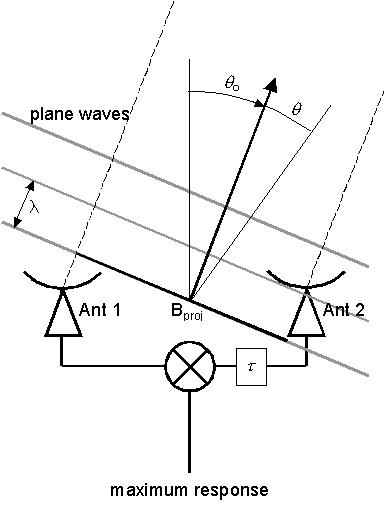
Figure 3: Geometry of an interferometer baseline where a delay t is
inserted in one antenna, in order to steer the phase center to a
direction q_o from the vertical l.

However, our expression (1) requires modification, since now it is the projected distance between antennas that matters, not the distance along the ground.  The fringe spacing is now given by

q = sin^-1l/B_proj   ~ l/B_proj                                               (2)

where we make the approximation that q is small and is expressed in radians.  Note that q  is now measured relative to the phase center direction, q_o.  The delay required to steer the phase center to the direction q_o is called the tracking delay, and must be continually updated to track the source across the sky.

The signal we have been discussing, with a maximum response at the phase center, is called the cosine component of the signal.  It is also possible to apply a phase shift of p/2 to the signal from one of the antennas and measure this new signal, called the sine component.  These two components are measured simultaneously.  Using the notation

x = cosine component
y = sine component

we can determine the amplitude of the wavefront as

a = (x² + y²)^1/2

and the phase of the wavefront as

f = tan^-1 (y/x) .

Point Source
Consider a point source in the sky, of amplitude a₁, located an angular distance q₁ = 10 arcsec from the phase center, as shown in Figure 4a.  When measured with a baseline whose fringe spacing is q = 30 arcsec,  the phase f₁ of this source will be f₁ = 2pq₁ /q  = 2p/3, which is the angle shown in Figure 4b.  The interferometer will measure a cosine component of x = a₁ cos(2p/3) = -a₁/2, and a sine component of y = a₁ sin(2p/3) = 3^1/2a₁/2.  These are the components of the vector shown in the phasor representation of Figure 4b, and can be written more compactly as

a₁ exp(if₁) = a₁ exp(i2pq₁ /q) .

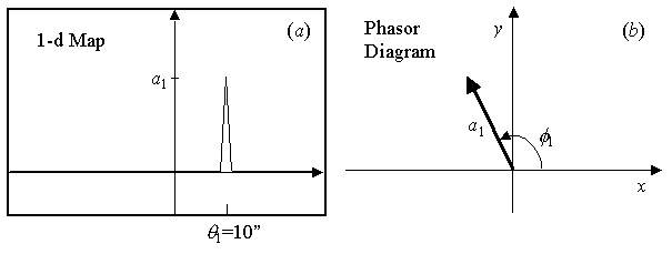
Figure 4: a) The spatial map of a point source of amplitude a₁ at spatial coordinate q₁.
b) The corresponding phasor diagram showing the interferometer response in terms of
the amplitude a₁ and phasef₁.

Two Point Sources
Now consider what happens when we add a second point source of amplitude a₂, located an angular distance q₂ = -2 arcsec from the phase center.  This is equivalent to adding another vector to the phasor diagram, with phase f₂ = 2pq₂ /q  = -2p/15, as shown in Figure 5.  Note that now the response of the interferometer is the vector sum of these two vectors, with resultant

a_r exp(if_r) = a₁ exp(i2pq₁ /q) + a₂exp(i2pq₂ /q),                       (3)

so the cosine and sine components are x = a_r cos(f_r), and y = a_r sin(f_r), respectively.

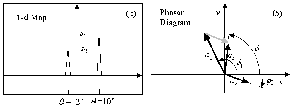
Figure 5: a) The spatial map of two point sources of amplitudes a₁ and a₂ at spatial coordinate
q₁=10" and q₂=-2". b) The corresponding phasor diagram showing the interferometer response
for the two sources, where the resultant of amplitude a_r and phasef_r is the vector sum of the two
individual responses.

A Continuous Distribution of Brightness
Any continuous distribution of brightness can be thought of as a collection of point sources.  Consider a source of gaussian cross-section,

a(q_i) = A exp(-[(q_i-q_o)/a]²) ,                                              (4)

where the q_i are the discrete spatial coordinates of size, say, Dq  = q_i -q_i-1= 1".  Figure 6 shows the spatial distribution of equation (4) for a 1/e width a = 5", centered at spatial coordinate q_o = 10".

 

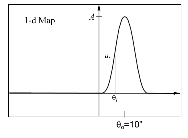
Figure 6: The spatial map of the gaussian function shown in eq. (4).  The amplitude and
position of one of the discrete 1" bins is shown.

By analogy with equation (3), it is obvious that the resultant signal measured by an interferometer baseline of fringe spacing q, will be

a_r exp(if_r) = S_ia_iexp(i2pq_i /q),                                            (5)

where the summation is over the discrete 1" spatial bins.  However, recall from Lecture 4 that the fringe spacing is the inverse of the spatial frequency, i.e. q = 1/s, and we identified coordinates u and v with the components of s, and the coordinates l and m with the sky components of angular position q_i.  Using these variables, equation (5) becomes

a_r exp(if_r) = S_ia_iexp[i2p(ul + vm)].                                     (6)

The Complex Visibility and Fourier Transform Relation
Finally, we define the response of the interferometer as the complex visibility, V(u,v) = a_rexp(if_r), define the sky brightness distribution as I(l,m) = a_i, and make the obvious generalization from a discrete summation to a continuous integral to obtain:
 

V(u,v) =		I(l,m) exp[-i2p(ul + vm)]	dl	dm .         (7)

Equation (7) demonstrates the Fourier Transform relationship between the sky brightness distribution I(l,m) and the interferometer response (complex visibility) V(u,v).  In particular, if we measure the interferometer response V(u,v), we can invert it (inverse Fourier Transform) to obtain the sky brightness distribution (the map):

I(l,m) =		V(u,v) exp[i2p(ul + vm)]	du	dv .         (8)

A synthesis imaging radio instrument consists of a number of radio elements (radio dishes, dipoles, or other collectors of radio emission), which represent measurement points in u,v space.  We now need to describe how to convert an array of dishes on the ground to a set of points in u,v space.

E, N, U coordinates to x, y, z
The first step is to determine a consistent coordinate system.  Antennas are typically measured in units such as meters along the ground.  We will use a right-handed coordinate system of East, North, and Up (E, N, U).  These coordinates are relative to the local horizon, however, and will change depending on where we are on the spherical Earth.  It is convenient in astronomy to use a coordinate system aligned with the Earth's rotational axis, for which we will use coordinates x, y, z as shown in Figure 7.  Conversion from (E, N, U) to (x, y, z) is done via a simple rotation matrix:
 

x

0

-sin l

cos l

E

y

=

1

0

0

N

z

0

cos l

sin l

U

which yields the relations

x = -N sin l + U cos l
y = E
z = N cos l + U sin l
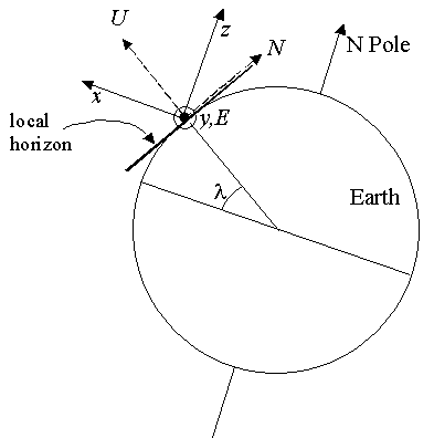
Figure 7: The relationship between E, N, U coordinates and x, y, z coordinates,
for a latitude l.  The direction of z is parallel to the direction to the celestial pole.
The directions y and E are the same direction.

Baselines and Spatial Frequencies
Note that the baselines are differences of coordinates, i.e. for the baseline between two antennas we have a vector

B = (B_x, B_y, B_z) = (x₂- x₁, y₂- y₁, z₂- z₁).

This vector difference in positions can point in any direction in space, but the part of the baseline that matters in calculating u,v is the component perpendicular to the direction q_o (the phase center direction), which we called B_proj in Figure 3.  Let us express the phase center direction as a unit vector s_o = (h_o, d_o), where h_o is the hour angle (relative to the local meridian) and d_o is the declination (relative to the celestial equator).  Then B_proj= B. s_o= B cos q_o.

Recall from Lecture 4 that the spatial frequencies u,v are just the distances expressed in wavelength units, so we can get the u,v coordinates from the baseline length expressed in wavelength units from the following coordinate transformation:
 

u

1

sin ho

cos ho

0

Bx

v

=

-sin do cos ho

sin do sin ho

cos do

By

w

l

cos do cos ho

-cos do sin ho

sin do

Bz

Notice that we have introduced a spatial frequency w, which we must include to be accurate.  However, if we limit our image to a small area of sky near the phase center (small angular coordinates l, m), then we can get away with considering only u,v coordinates.  Ignoring w causes distortion that is akin to projecting a section of the sky dome on a flat plane, as shown in Figure 8. The condition for this to be valid is 1/2 (l² + m²)w << 1.  For w = 1000 wavelengths for example, we could map out to about 1/30 radian or a little over 1 degree.  As we use higher frequencies and/or longer baselines, the part of the sky we can map without distortion gets smaller.  We will henceforth ignore the w coordinate and assume that we are measuring the sky in a small region near the phase center.

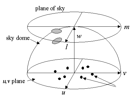
Figure 8: The sky dome and its approximation as a flat "plane of the sky" are shown.
For baselines with a significant w component, the approximation of a flat sky causes
distortions near the edges of the map.  The gray oval on the plane of the sky is really
on the curved sky dome.

Note that u,v depend on the hour angle, so as the Earth rotates and the source appears to move across the sky, the array samples different u,v at different times.  Figure 9 shows an example with antenna locations (9a), the corresponding u,v points at a single instant in time (9b), and the u,v points over many hours in time (9c).  The u,v points trace out portions of ellipses, called u,v tracks, and sample more of the u,v plane.  Making a map over a long period of time is called Earth Rotation Synthesis.

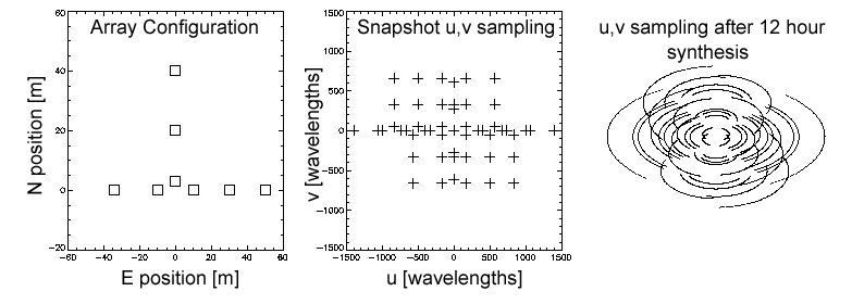
Figure 9: a) An example array configuration consisting of 8 antennas, with E and N antenna locations in meters.
b) The u,v sampling that results from this array for a single time (snapshot), at zero hour angle.  Each cross represents
a baseline.  There are N(N-1)/2 = 28 unique baselines, but there are twice this many points due to symmetry.
c) The u,v sampling that results after a 12 hour integration.  The rotating Earth causes the projected baselines
to change with time, tracing out portions of elliptical paths.

The way to think about the problem is to consider that for every sky brightness distribution I(l,m) there exists a visibility function V(u,v) that is its Fourier Transform.  This visibility function is everywhere a continuous complex function.  An array of antennas with baselines B_l,proj = (u_i,v_i) measures only certain values in the set of continuous (u,v) in the visibility function. This measured set we call the sampling function S(u,v) = S_kd(u - u_k,v - v_k).  Here d(x,y) is the 2-d delta function, and the sum is taken over all baselines.  The sampled visibility function S(u,v)V(u,v) is the actual data provided by the array, and by performing the inverse Fourier Transform we recover the "dirty image" I_D(l,m), given by

ID(l,m) =		S(u,v)V(u,v) exp[i2p(ul + vm)]	du	dv .         (9)

Note that the dirty image uses only the sampled visibilities, and so does not contain full information about the sky brightness distribution.  We must use some image reconstruction technique to recover the missing spacings.  Note also that the actual visibility function measured by the instrument is V'(u,v) = V(u,v) + N(u,v), where N(u,v) is an unavoidable noise component.

We could use a "brute force" method and calculate the dirty image via the direct Fourier Transform, but this would require 2MN ² multiplications, where M is the number of samples (baselines*times, or u,v points) and N is the linear dimension of the image, in pixels.  In practice, M ~ N (to fill the u,v plane), so multiplications (and sin/cos evaluations) go as N ⁴.

Instead,  we use the FFT, which requires of order (N ² log₂ N) operations, but to use this requires gridding the u,v data, which we will discuss in more detail shortly.

Sampling Function
Recall the convolution theorem, which states that the Fourier Transform of a product of two functions is the convolution of the Fourier Transforms of the individual functions, and vice versa.  If we denote the FT of a function F as F, then

AB = A * B                            (convolution theorem)
A * B = A B .

where the * symbol denotes convolution.  Application of the convolution theorem shows that

I_D = S(u,v)V(u,v) = S(u,v) * V(u,v)

which can be interpreted as saying that the FT of the sampling function, S(u,v), is convolved with the brightness distribution V(u,v).  We identify the FT of the sampling function, S(u,v), as the synthesized beam, or point-spread-function (PSF), or diffraction pattern of the aperture:

S(u,v) = B(l,m)

(not to be confused with the baselines, B_l,proj). We obtain by the synthesized beam by filling in our sampled u,v points with real part = 1 and imaginary part = 0.  This is exactly what we did with our exploration of the primary beam pattern for a single dish, if you will recall.  Note that B(l,m) is also the image we would obtain if we observed a unit point source at the phase center, since d(l,m) = V(u,v) = 1 + 0i, and

I_D = B = S(u,v)V(u,v) = S(u,v) * d(l,m) = S(u,v)

Note that this result is very general, and works just as well for optical systems, where the sampling function is called the point-spread-function.

As we noted above, we invert the sampled visibilities to obtain the dirty image.  We will do an example in class, to demonstrate the relationships shown in Figure 10.  The upper row are the sky plane (l,m) representations of map, beam, and dirty map.  The lower row are the corresponding u,v plane representations of visibility, sampling function, and sampled visibility.  Panel (f) represents the actual measurements made by a radio array.  Panel (c) represents the actual image from the array.  There are standard image reconstruction techniques, which we will discuss next time, that essentially try to predict the missing visibilities in panel (d), to arrive at the true map (a).

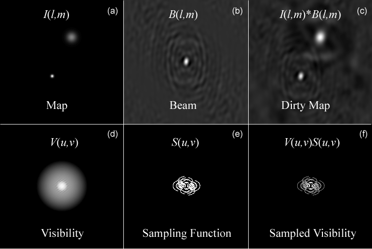
Figure 10: a) An example (model) sky map. d) The corresponding visibilities (Fourier Transform of the map).
c) The synthesized beam, or point-spread-function, of a model antenna array.  e) The sampling function of the
array, whose Fourier Transform gives the beam in (b). f) The product of panels (d) and (e), representing the
sampled visibilities.  These are the actual measurements from the array.  c) The dirty map that results from
the Fourier Transform of the sampled visibilities.  This is the same as the convolution of the map in (a) and the
synthesized beam in (b).

Weighting Functions and Beam Shape
As with any image processing, it is possible and sometimes desirable to use weighting to control the point spread function.  The synthesized beam may have large positive or negative sidelobes (the irregularities away from the center of Figure 10b) that we would like to minimize.

There are two important types of weighting commonly used in radio astronomy, called tapering and density weighting.  Tapering is used to suppress small-scale variations in the dirty map caused by incomplete sampling on the longest baselines (the largest u,v spacings).  Often a gaussian taper

T(u,v) = exp[-(u² + v²)/s²]

is used, where s is a measure of the width of the taper.  Note that the shape of the beam is improved at the expense of spatial resolution.  This is analogous to smoothing, and is also used routinely in optical image processing.  Other forms of taper can be used--even "negative taper" where the outer u,v points are enhanced to improve spatial resolution.

The other important type of weighting is density weighting, in which the weighting factor is proportional to the number of u,v measurements in a given gridded cell.  Two common choices are

D_k = 1                 Natural weighting
D_k = 1/N_S(k)        Uniform weighting

where D_k is the weight to be applied to cell k, and N_S(k) is the number of samples falling into cell k.  It is typical for arrays to have a much larger number of short baselines that long ones.  This is especially true of the Nobeyama array, which has a huge number of baselines of length d, and only a few larger ones:

. . . . . . . .   .   .       .       .       .
|--4d---|     |--4d---|       |--4d---|          Lots of 4d spacings
|--------------------23d----------------------|  Only one 23d spacing

This is made worse by the rate of angular change in the u,v plane when integrating over some time.

As a rule, uniform gridding gives the more pleasing result, with the full resolution of the array.  However, when mapping an extended source a natural weighting gives smoother extended emission by minimizing the negative inner sidelobes.  Other techniques can be used in later image reconstruction to influence the resolution and sensitivity to extended emission, which we will cover next time.

Gridding
In order to use the FFT algorithm, the measured u,v points must be gridded into the 2-d array to be inverted.  As it turns out, the precise way in which this is done can greatly affect the macroscopic properties of the resulting image.  The procedure can be thought of as a convolution, and we now look at some gridding convolution functions C(u,v).

1. Pillbox
2. Truncated exponential
3. Truncated sinc function
4. Exponential times truncated sinc
5. Truncated spheroidal

These are truncated of necessity because they involve examining a range of FFT cells and seeing which u,v points lie within the search range--typically 6 or 8 cells.  Each is truncated to
a width of m cells so that

C(u) = 0 for |u| > mDu/2.      where Du is the u,v plane cell spacing.

• Pillbox

C(u) = 1 for |u| < mDu/2
           0 otherwise

This is equivalent to "nearest neighbor" if m = 1, and one simply sums the data in each cell.  This is the fastest algorithm, but suffers the worst aliasing problems.  Remember that C*V = C V, so the image V is multiplied by C, which for a pillbox is just a sinc function.
 

• Truncated Exponential

C(u) = exp[-(|u|/wDu)^a]
where typically m = 6, w = 1, and a = 2 (gaussian).  Then C is also a gaussian and falls off as a gaussian outside the map.

• Truncated Sinc

C(u) = sinc(u/wDu)
where typically m = 6, w = 1.  If we use a width m = width of the map (expensive in compute time!), then C is a square wave and falls off sharply, which is the justification for this functional form.

I will not go through the others, but one can see that gridding is an important part of inverting the measurements to get the cleanest possible image.  Again, gridding is forced upon us by use of the FFT.  It completely disappears if we use the discrete Fourier Transform.

Define

V(u,v) = actual visibility function
V ' (u,v) =  measured (i.e. noisy) visibility function
W(u,v) = T(u,v) D(u,v) = weighting function, including both taper and density weighting
C(u,v) = gridding convolution function
R(u,v) = Resampling function (bed of nails function, representing pixelization)

R(u,v) = III(u/Du,v/Dv) = S_jS_kd(j- u/Du, k- v/Dv)

The final resampled visibility function is

V_R = R [C * (WV ' )]

and after FFT we obtain the "dirty image"

I_D = V_R = R * [C (W * V ' )]

The convolution with R is the step that causes aliasing, so we choose a gridding convolution function C(u,v) that minimizes aliasing.