The first part of
the receiver is the heterodyning to bring the RF (radio frequency) down
to a manageable intermediate frequency (IF) that we can work with.
This requires a mixer and local oscillator (frequency reference), as shown
in Figure 1, below:
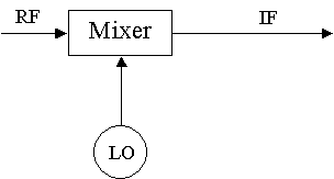
Figure 1: Heterodyne
receiver, which uses a local oscillator (LO)
operating at frequency wo,
to tune to the desired radio frequency (RF)
and mix with RF at a wide
band of frequencies, and strip off a lower
bandwidth section of intermediate
frequency (IF) for further processing.
For interferometry, we must
correlate the signals from two antennas, which requires a number of additional
considerations. The main one is to ensure that the receivers of
the two antennas are operating at exactly the same frequency. If
one were on a frequency different by only 1 Hz, the resultant phase between
the two would change by 360 degrees every second! In the past, it was
not possible to transmit a broadband signal from each antenna, which meant
that the signal at each antenna had to be mixed down to a lower frequency.
That required the use of a reference signal sent to each antenna. Figure 2
shows an example of such a scheme. To control the frequency, a phase lock system
was used as in Figure 2.
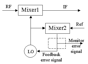
Figure 2: Adding
a phase lock loop, which compares the LO output
with an external reference
frequency and sends an error signal back
to the LO to keep it in
perfect phase lock with the reference signal.
Each antenna receives the
Ref signal from the same source, so all
receivers are locked to
the same frequency.
Mixer 2 compares the LO to
a frequency reference, which comes from the same frequency source for all
antennas. Any error in the phase results in an error signal that
is fed back to the oscillator to adjust its frequency to maintain exact
frequency tuning.
With modern technology, it is now possible to transmit
broadband signals via optical fiber. The EOVSA system, for example, transmits two 1-18 GHz RF signals
multiplexed onto a single optical fiber to the central control room. In the confined space of the
control room, it is possible to distribute the local oscillator signals directly to the 15
downconverter modules and avoid the need for a distributed phase lock system.
Let's look at what happens to the signal after it leaves the EOVSA front end
and enters the receiver. The figure below is the block diagram for a downconverter module in the Expanded Owens Valley Solar Array.
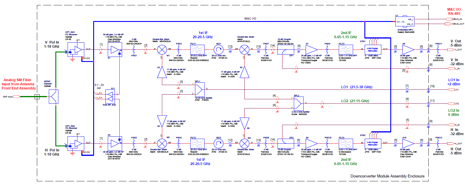
This is a dual-channel receiver,
with H pol and V pol signals being received separately on optical fiber. The signals enter
on the left and exit on the right. The signals are converted to electrical form, go through two stages of frequency conversion, which selects a 400 MHz intermediate frequency (IF) portion of the incoming 1-18 GHz radio frequency (RF), adjusts its power level by means of amplifiers and attenuators, and then provides this clean 400 MHz IF to the digitizers in the correlator chassis (not shown). Click this link for a description of the EOVSA downconversion and frequency tuning.
The IF signal from
each receiver looks like a noise signal. Part of the waveform is
really signal from the source, and part of it (perhaps the largest part)
is noise. If both signal and noise look the same, how do we tell the difference?
The essential point is that source signal will be correlated between the two antennas, while the
(locally generated) noise signal will not. This is illustrated with the simulated waveforms
from two antennas, below:
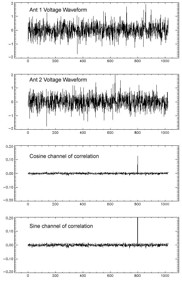
Figure 3: Two simulated
voltage waveforms, with phase 30 degrees, with the
waveform for antenna 1 shifted
by 800 time samples. The noise level is 1/5 of
the signal level in this
example. The waveforms appear to have no relation to
one another, but when correlated
they give the plot in the third panel (cosine
channel), which shows a
good correlation (spike) at a time lag of 800 samples.
Shifting the antenna 1 waveform
by 90 degrees and performing the correlation
again gives the result shown
in the bottom panel (sine channel). The combination
of the sine and cosine channels
gives an amplitude of 0.268 and phase of
30.2 degrees. The
correct values are 0.25 and 30 degrees.
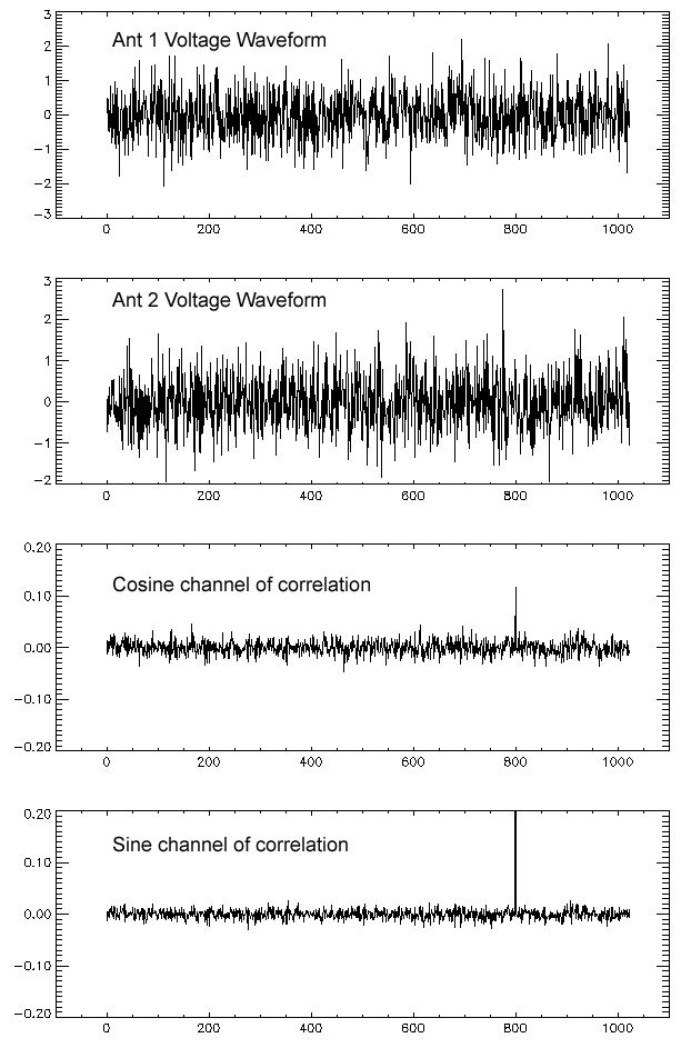
Figure 4: Two simulated
voltage waveforms, with the same characteristics as for
Figure 3, but now the noise
level 5 times higher and is now equal to the signal level.
Because the noise is uncorrelated,
the correlated signal is hardly affected, and gives
and amplitude of 0.245 and
phase of 30.83 degrees, compared to the correct
values of 0.25 and 30 degrees.
Given time varying voltages V1 and V2,
the correlation is found by multiplying them, with one delayed by the geometrical
delay tg= B . s/c, then averaging, i.e.
r = <V1(t)V2(t)>
where < >
denotes the expectation value, found
by averaging over some integration time. Considering for the moment
a monochromatic time-varying signal
V1(t)
= v1 cos[2πν(t−τg)]
V2(t) =
v2
cos[2πνt]
we have
r = <v1v2
cos[2πν(t−τg)]
cos[2πνt]>
= v1v2
<cos2(2πνt)
cos(2πντg)
+ cos(2πνt) sin(2πνt)
sin(2πντg)>
= v1v2
cos(2πντg)
Since the geometrical delay
τg
changes due to the Earth's rotation, the relatively slowly varying cosine
term causes the oscillations that represent the motion of the source through
the interferometer fringe pattern. In the old days of chart recorders,
this fringe pattern was traced on paper and its amplitude and phase could
be measured by hand. The rate of fringe oscillations is called the
natural
fringe rate. The fringe frequency is
νF
= dw/dt = −Ωe
u
cos δ
where Ωe
is the Earth rotation rate, w = (Bλ
. s) is the spatial
frequency corresponding to the projected baseline z-component
given by the coordinate transformation from the previous lecture, u
is the usual E, or y-component
spatial frequency, and δ
is the declination of the phase center. The geometry is as shown
in Figure 5.
Figure 5: The geometry
and block diagram leading to the measured cosine component
of the correlation.
Both the multiplier and the integrator are part of the device called the
correlator. A refinement
is shown in Figure 6.
A major refinement is to
use a second correlator, and shift one of the signals by π/2, so that both
sine and cosine components are measured simultaneously, as shown below.
The components in the dashed box in Figure 5 are indicated by each circled
X in Figure 6.
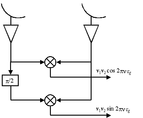
Figure 6: Inserting
a phase shift of π/2
in one of the antennas and doing a
second correlation allows
both sine and cosine components to be measured
simultaneously. These
are recorded and become the complex visibility at
spatial frequency u,v
corresponding to the projected baseline between the
antennas.
The quantities measured out
of the correlator are the real and imaginary parts of the complex visibility
measured with the baseline, whose normalization is obtained by the calibration
procedure, which we have not yet discussed. You may wonder how we
accomplish the 90 degree phase shift over a finite IF bandwidth Δν.
This was done in the old OVSA receivers by changing the phase of the reference
signal used to phase lock the local oscillator. Note that this is
not equivalent to a time delay, which would shift the phase by different
amounts for different frequencies, but rather it shifts the phase of each
frequency separately. In the new EOVSA system, we use the digital correlator to
do the phase shifting. As it turns out, phase shifting, or synchronous
detection, is also important for eliminating any DC offsets. If we
multiply two waveforms with a DC offset, the offsets will give a non-zero
signal even when there is no correlation in the signals. This is
eliminated by periodically inverting the signal at the antenna, and then
synchronously inverting the signal again at the correlator. In this
way, the signals stay correlated while any unwanted DC offset gets inverted
periodically and averages to zero.
To discuss correlators further,
we will use the NRAO Summer School lecture
on cross correlators.