When I was first studying planetary systems, we had exactly one example--our own solar system. In October 1995, the first extrasolar planet discovery was announced: a planet orbiting the star 51 Pegasi (Mayor and Queloz). Within a few months, Marcy and Butler announced the discovery of planets around two other stars. This launched a flurry of planet detections that continues at an every accelerating rate to this day, and promises to continue well into the future. In this lecture, we will examine the techniques, current status, and summarize the discoveries made to date.
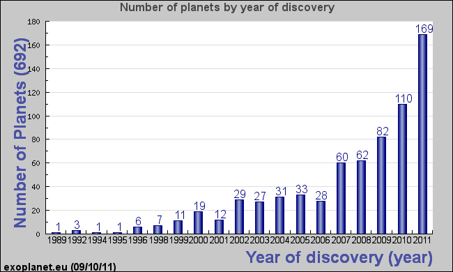
To give you an idea of the rate of discovery, currently there are a total of 692 announced discoveries. A space mission dedicated to discovering exoplanets (extrasolar planets) is the Kepler mission, which has announced 1236 additional candidates that are being studied to verify their status as planets. Note that reports earlier than 1995 are either planets around non-normal stars (pulsars) or were confirmed later than 1995.
Some reasons for the explosion of discoveries are the development of new instruments/detectors, refinement of techniques for detection, the development of new methods of detection, and the increase in number of groups now actively working on discoveries and follow-up observations. Below is a similar plot as the above, but with discovery methods indicated.
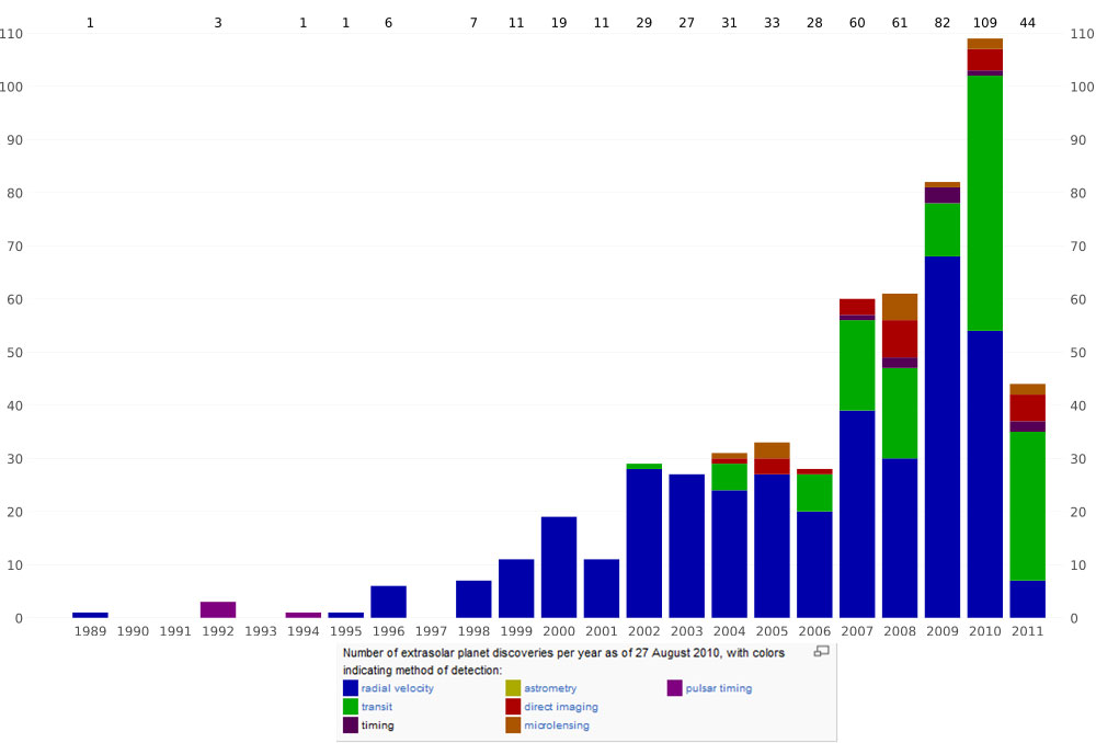 |
| Plot of exoplanet discoveries versus year of discovery, color-coded by method of discovery. The 2011 bar is incomplete. Two methods are the dominant ones, the radial velocity method and the transit method. This plot is adapted from Wikipedia. |
B. Methods of Detection
Radial Velocity Method
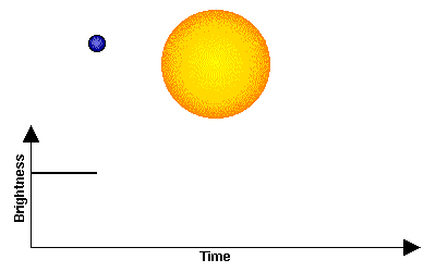
The most prolific method of detection is by measuring the radial velocity of the star that the planet is orbiting around. We discussed earlier that two bodies can be thought of as orbiting their common center of mass (barycenter). The planet is undetectable, but the star is easily seen, and should show a wobble about a point not quite at its center. The period of the wobble is exactly the same as the period of orbit of the planet. To measure the period, and the extent of the wobble, we can use measurements of doppler shift of spectral lines to measure the "radial velocity" (the speed with which it is either moving towards us, causing a blue shift in spectral lines, or away from us, causing a red shift). The figure below shows the physical situation, and the link is to an animation that shows the corresponding shift in spectral lines.
 |
Wobble in position of a star caused by gravitational effect of a planet orbiting around it. The two objects, planet and star, each orbit about a common point that is the center of mass of the system (the barycenter). See this link for a video of the doppler effect on spectral lines (vastly exaggerated--the actual shift of spectral lines is extremely tiny and difficult to measure). |
The text notes that radial velocities as small as 3 m s-1 can be measured, about the speed of a slow jogger. Marcy, Butler and colleagues pass the starlight through an iodine vapor, so that they record both the "rest wavelength" of the iodine lines and the wavelength of the corresponding iodine lines in the star spectrum. Of course, we must keep track of many other motions, for example the Earth's spin and wobble, motion of the Earth around the Sun (30 km s-1), and the motion of the Sun relative to the star. Other motions on the star itself also have to be considered, such as its own rotation, possible oscillations or pulsations (in and out motions) of the star's surface. For reference, would the planets in our solar system be detectable by this method, if the limit is 3 m s-1? This is given as a homework problem. Note that the masses of planets determined by the radial velocity method are actually lower limits (M sin i, where i is the angle of inclination of the orbit from the plane of the sky). The reason is not hard to see. Imagine that the figure above is seen from "above" as shown. The motion of the star is entirely in the plane of the page, so there is no radial velocity. The inclination in this case is i = 0 (the orbit is in the plane of the sky), so sin i = 0. When viewed from the side, i = 90 degrees, so sin i = 1. The mass estimate is Mest = M sin i, which is a lower limit to the true mass, M.
Transit Method
The next most prolific method, and one that is destined to overtake the radial velocity method, is detection by measuring a decrease in brightness of a star due to the passage (transit) of a planet in front of the star. The basic method is shown in the figure below, but note that the planet is often very small compared to the star, so the decrease in brightness is often extremely small, perhaps 3-4 millimagnitudes for a large planet, grading down to indetectability for small planets.
 |
Transit of a planet in front of a star, and the effect on the overall light coming from the star (transit light curve). |
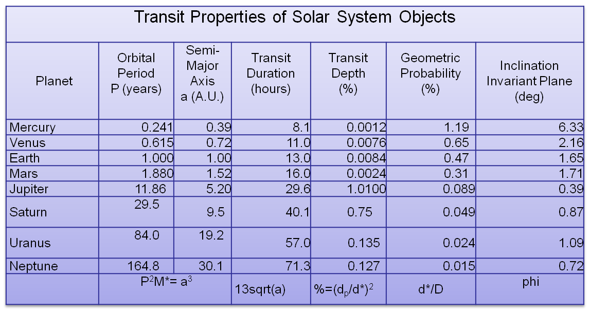
To get a feeling for the detectability of planets by the transit method, the table below shows the transit properties of the solar system. If you were observing our Sun from another star, and happened to be aligned such that the inclination angle was close to 90 degrees, you would detect transits of the planets as shown. For the Earth, for example, once per year you would see a dip of 0.0084% of the brightness of the Sun (or a factor of 0.000084). If the flux of the Sun is considered to be 1 without the transit, then during the transit the flux would be 0.999916, so the magnitude change (m1 - m2 = 2.5 log f2/f1 = 2.5 log 0.999916 = 0.01 millimagnitudes). We can conclude that detecting Earth from another star would be very hard! How about Jupiter? The change in magnitude during a transit would be much larger, about 11 millimagnitudes, which is easily detectable, but the dip would only occur once every 11.86 years, and we would have to be much better aligned (inclination angle within 0.39 degrees of 90).
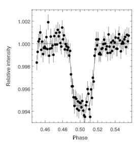
The figures below show an example of an infrared transit, and what can be measured with combinations of optical and infrared transits.
 |
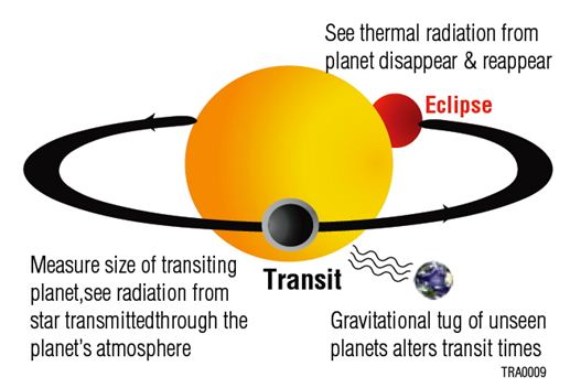 |
| The light curve at left is a transit in the infrared (IR) detected by the Spitzer spacecraft. Note that the depth of such transits can be very large (0.6% in this example) because the star is not as bright, and the planet can be very bright in the IR. At right is a diagram showing some of the ways transits can be used. |
The Kepler Space Mission
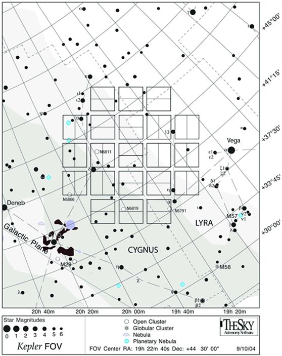
One reason that transits are destined to become the more prolific method of detecting new objects, at least for awhile, is the recent launch and continued operation of the Kepler space mission. Kepler is in orbit about the Sun, and staring at a single region of the sky in the constellation Cygnus.
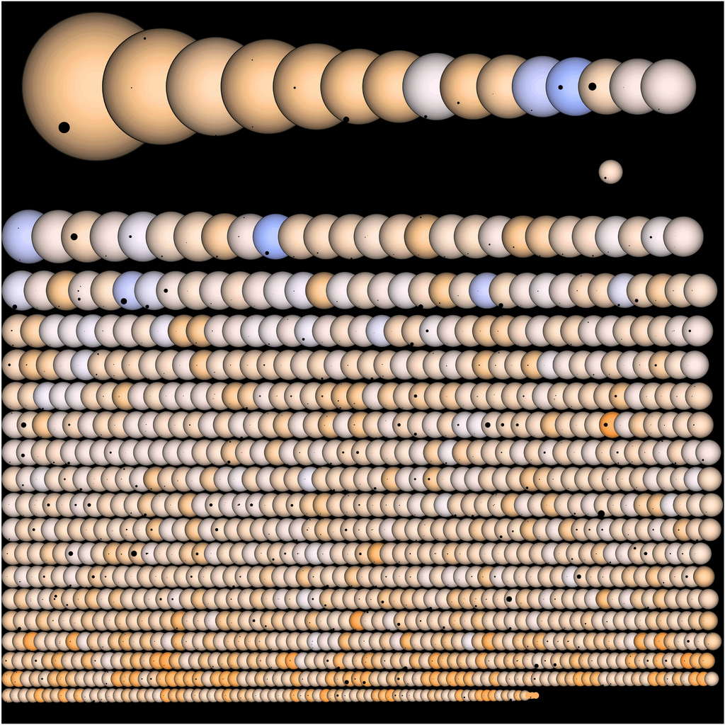
Kepler is viewing more than 100,000 stars at once, taking high-precision, low-noise measurements of each one for up to four years. An extended mission of an additional two years is hoped for. Let's take a look at the data for one particular object (you can select any of the other 1236 candidate objects and look at their light curves). http://archive.stsci.edu/kepler/data_search/search.php?action=Search&ktc_kepler_id=8030148. Selecting the second light curve brings up the data, which you can plot at different resolutions. A clear dip in brightness is occurring every 6 days or so, with a fractional dip of 0.0006. If you explore other sections of the data for the same object, you may see other dips. Could these be other planets? In order to know for sure, you would have to have at least three dips due to the same object, separated by the same orbital period. That means the Kepler cannot verify planets with periods less than about 1/3 of its 4-yr mission duration (1.3 year periods).
C. Characteristics of Extrasolar Planetary Systems
Even though the text we are using, Carroll and Ostlie 2nd Edition, is a recent edition published in 2007, it is already woefully out of date with regard to the rapid increase in knowledge of extrasolar planetary systems. I have updated some of the information in this lecture, but by a year from now this lecture, too, will be out of date. Still, here is what we know so far about other solar systems.
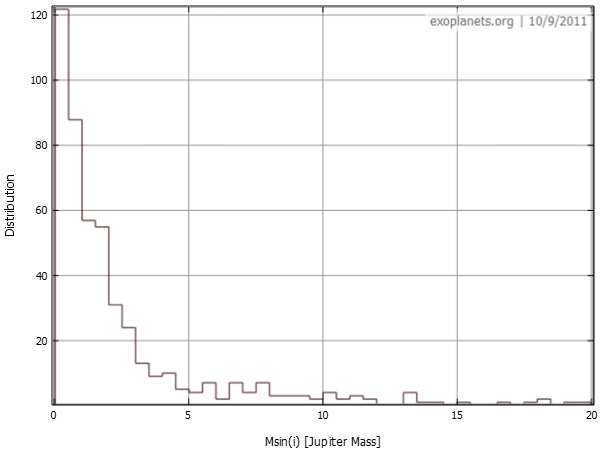

|
| Two plots of the histogram (number of planets vs. mass, or M sin i). Note that the units are Jupiter masses. The upper plot (exoplanets.org) is a linear plot, while the lower plot (exoplanet.eu) is logarithmic in mass, emphasizing the mass distribution below 1 Jupiter mass. |
The orbital parameters of the known planets are shown in the next series of plots, semi-major axis, inclination from the plane of the sky, and eccentricity. You can see that the orbits come in all types.
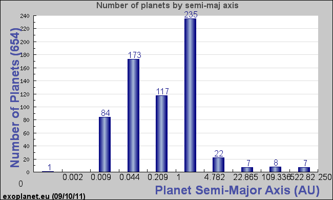 |
| Distance of the planet from the parent star (semi-major axis a), shown logarithmically in AU. Note that many of the known extrasolar planets are much closer in than the planets in our solar system, and some of them are very large (larger than Jupiter--see mass vs. a plot below). Why do you think that may be? |
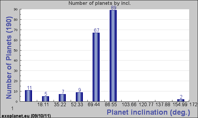 |
| The inclination of the orbit from the plane of the sky (those in the plane of the sky will have zero inclination, and those seen edge on will have 90 degree inclination). Most of the known extrasolar planets have very high inclinations. Why do you think that is? Note that only 190 of the 686 known planets are shown--the others do not have measured inclincations. |
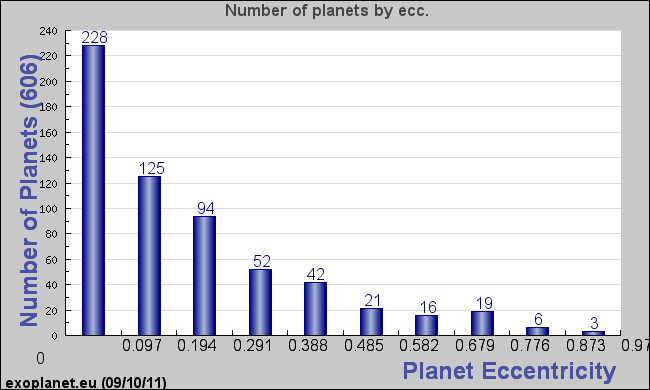 |
| The eccentricity of the orbits of 606 extrasolar planets, shown on a logarithmic scale. Note that most orbits are fairly circular, but many are quite elliptical. What do you think the radial velocity curve would look like for elliptical orbits? |
The physical properties of the known extrasolar planets is also quite interesting. Below are some plots of planet mass, radius vs. mass, and mass vs. semi-major axis.
|
| The mass of the known extrasolar planets, on a logarithmic scale, in units of Jupiter masses. Most are at least the mass of Jupiter, and some are much larger, nearly the mass limit of brown dwarfs (~13 MJ). Note that one Earth mass is only 0.003 MJ, so only a handful of planets are anywhere as small as 1.3 Earth mass. Why do you think that might be? |
|
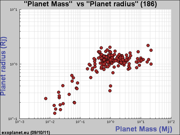
| For the 186 exoplanets for which both mass and radius is known, the above plot shows that mass and radius are correlated up to about 0.4 MJ, and then the radius becomes nearly constant with increasing mass. Recall that we said brown dwarfs are not much bigger than Jupiter. What do you think is happening here? |
|
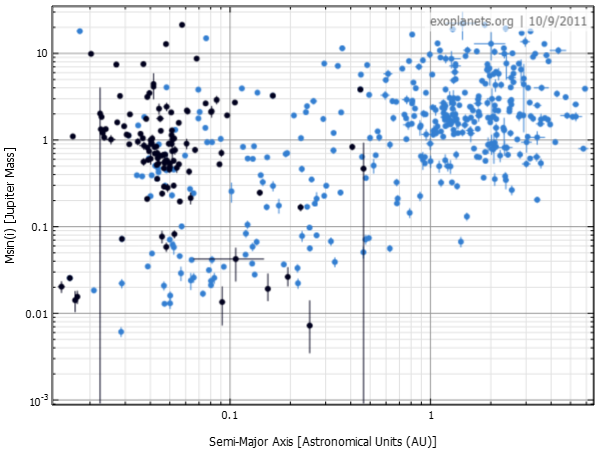
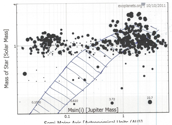
| This is a plot of mass (M sin i) vs. orbital distance (semi-major axis a). The objects shown with blue dots were detected using the radial velocity method, while those with the black dots were discovered using the transit method. Why do you think the transit method (so far) is unable to detect planets farther from the parent star? The large, close-in objects are called "hot Jupiters," and there is a strong selection bias for finding such planets. |
|
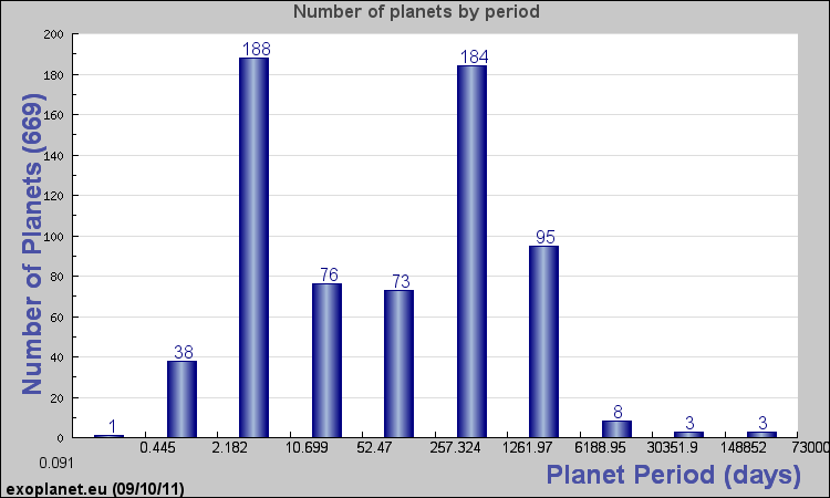
| The orbital period of exoplanets, on a logarithmic scale. Note that there are two peaks, one due to detection by the transit method and the other due to detection by the radial velocity method. The selection bias in our detection methods produce skewed results, so one must continually be aware of that. |
The main reason the transit method is not good at detecting more distant planets is that it takes time to see transits of planets with an orbital period of a year or more. The search has just not been running for long enough, but if Kepler or similar missions run long enough, we should be able to find planets with longer orbital periods and fill in the distribution.
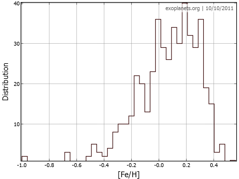
Finally, it is interesting to consider what kind of star exoplanets are found orbiting around. The ratio of iron (or metals) to hydrogen is an important measure of the original constitution of the protostellar cloud. It should make sense that clouds with lots metals should make more and bigger planets. The plot below shows the number of exoplanets vs. log of Fe/H ratio, with log(Fe/H) = 0 for our Sun. Stars with negative log(Fe/H) are metal deficient relative to the Sun, while positive values are metal rich.
|
| The number of exoplanets vs. log of Fe/H ratio, with log(Fe/H) = 0 for our Sun. Stars with negative log(Fe/H) are metal deficient relative to the Sun, while positive values are metal rich. |
D. Summary of Extrasolar Planet Characteristics
Again, we should always be aware of the selection effects of our detection methods, and be careful not to make an incorrect generalization based on incomplete data. But we can say that the known systems have the following properties:
- Planets are quite common around stars with high metalicity (high Fe/H ratio), perhaps as much as 25% of stars have planets of Jupiter mass.
- The planets do not follow any clear progression of planetary size and location, as the planets seem to do in our solar system.
- Many of the known systems have hot Jupiters, which are a surprise and a challenge for theories of solar system formation. Did they form there, or did they move there after forming elsewhere?
- A sizeable number of stars have more than one planet known (and it is expected that most do).
It is of interest to ask whether any of the known exoplanets could harbor life, and especially whether they could support humans. Some clearly are too large and too hot to be habitable to humans, but of course life can come in many varieties, so the question of life is a more complicated question. We should keep in mind that even those that are too large for humans could have moons that might be perfect for us if they are not too hot or too cold. We can find the comfort zone (habitable zone) by considering where liquid water could exist. See the plot below.
|
| A depiction of the habitable zone within which liquid water can exist on a planet is shown by the hatched area. This is a matter of distance from the parent star, and the brightness of the parent star (related to its mass). Many planets fall within the habitable zone, but all (so far) are much bigger than Earth (one or two are only slightly bigger, but so far no Earth size or smaller world has been found in the habitable zone). However, considering the case of Jupiter, large planets can have sizeable moons that could be habitable. |