Power vs. Temperature

The power level of the radiation (W) can be traced from its reception by the feed, through the receiving system.  The "signal" is generally noise-like (white noise, containing all frequencies in the band).  For convenience, which will become clear, we often consider the equivalent noise temperature corresponding to the power level

P = kT Δν

although we also refer to the power level in decibel milliwatts [dBm].

We can consider the power received by the antenna,

P_a = kT_aΔν,                                                 (1)

where T_a is the antenna temperature, and the output power of the receiver as

P_tot = P_a + P_sys => T_tot = T_a + T_sys ,

where T_sys is the system temperature, and represents the added noise of the system.  It is a figure of merit, and should be kept as low as possible.  We can break the system temperature into several contributions:

T_sys = T_bg + T_sky + T_spill + T_loss + T_cal + T_rx ,
             lump into T_a           lump into T_rx

where

T_bg = noise contribution from microwave and galactic backgrounds
T_sky = noise contribution from atmospheric emission
T_spill = noise contribution due to ground radiation (spillover and scattering)
T_loss = noise contribution due to losses in feed
T_cal = noise contribution due to injected noise
T_rx = receiver noise temperature

To give you an appreciation for the magnitude of these contributions, the following table gives the VLA performance as an example:
 

λ	Tbg	Tsky	Tspill	Tloss	Tcal	Trx	Tsys
92 cm	25	3	15	7	5	70	125
20 cm	3	3	14	8	2	30	60
6 cm	3	3	7	5	2	30	50
3.6 cm	3	2	5	2	2	16	30
2 cm	3	8	6	13	6	80	116
1.3 cm	3	17	6	21	7	100	154

• Note: T_bg , T_sky , and T_spill  vary with position on the sky.

• T_bg  is the 3 K cosmic background (leftover emission from the Big Bang), except at the lowest frequency where radio emission from the galaxy becomes important.

• T_sky = T_sky(1 − e^−τo^{csc E}), where τ_o = zenith opacity, E = elevation angle.  The value of T_sky is generally small except at high frequency where the atmosphere beocmes more opaque.

To see how important the unwanted T_sys is, let's compare it with a typical signal.  Say we have a point source of flux density 1 Jy [= 10⁻²⁶ W m⁻² Hz⁻¹].  If observed with a radio telescope of 10 m diameter, what is T_a?

S = 2kT_aν²/c²Δν .                                                  (2)

Note that ΔΩ > ΔΩ_source  so use ΔΩ_beam.  From θ_FWHM ~ λ/D

ΔΩ_beam = π/4 (θ_FWHM)² = π/4 (c²/D²ν²)                   (3)

Insert (3) into (2) and solve for T_a,

T_a = Sc²/2kν² 4/π (D²ν²/c²) = 4SD²/2πk = 4(10⁻²⁶)(10²)/2π(1.38 x 10⁻²³) = 0.04 K!

So in order to measure a 1 Jy source, we have to measure 0.04 K against of order 100 K of system noise.  If we make the antenna more directive (D larger) then the situation improves.  The 100 m Bonn telescope, or the GBT antenna would see 4 K from a 1 Jy source.  The 1000 ft Arecibo dish would see ~40 K.  However, recall from last time that the effective area of an antenna is reduced by the efficiency, A = ηA_o, with η ~ 0.5, so the problem is even worse.  The appropriate antenna temperature expression for a source of flux density S is

T_a = SηA/2k.                                                  (4)

so Bonn has 1.5 K/Jy, Arecibo: 15 K/Jy.  Clearly we are measuring very small signals.

We can take advantage of the fact that the signal will be correlated from one sample to the next, while the noise will not be, and "beat down the noise" by making many sample measurements and adding them up.  According to the Nyquist theorem, a time series of measurements of signal of bandwidth Δν, of duration τ,  will contain 2Δντ independent samples, so the noise should go down by the square-root of the number of samples, or

ΔT = T (2Δντ)^−1/2 ,                                         (5)

where T is the equivalent temperature of the signal plus noise.  A more general expression, from Crane and Napier (1989) and Anantharamaiah (1989) [an earlier version of the NRAO Summer School book] is
 

ΔT =[	Ta2 + TaTsys + Tsys2/2	]	1/2	(6)
	Δντ

Normally when observing cosmic sources, we can ignore T_a relative to T_sys , which reduces to equation (5) with T = T_sys.  However, what happens when we observe a strong source such as the Sun?  The brightness temperature of the quiet Sun is about 10,000 K at, say, 10 GHz (recall homework problem set #1), so if we observe the Sun with a 25 m antenna with aperture efficiency ~ 0.5, the 10,000 K source will fill the beam and the antenna temperature will be 5,000 K.  This is now much larger than the typical system temperature, so we say that the source dominates the noise, and the sensitivity of the antenna is now less than before.  We will revisit this when we examine the sensitivity of an interferometer, and discuss the minimum noise level in radio images.

Let us now examine the signal path from the feed to the receiver.  This chain is called the front end, and its characteristics dominate the noise of the system.  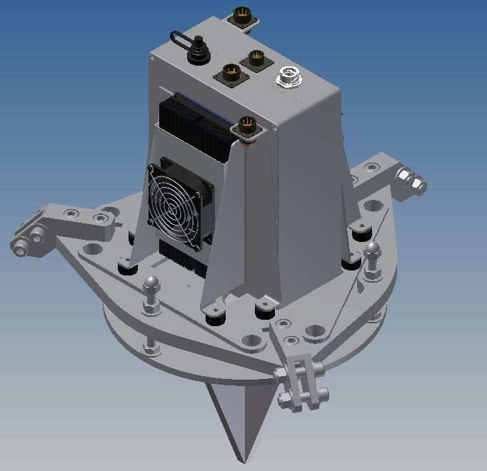A typical front end consists of the feed, some connecting cables, perhaps with filters or couplers, then a first stage low-noise amplifier (LNA), then typically a second stage LNA, followed by the receiver itself, as shown in the schematic below: A front end that I built for Lucent Technologies (the Solar Radio SpectroPolarimeter) is shown in the figure below left, while the EOVSA front end is shown below right:

Before considering individual elements, we develop the concept of a general 2-port device, as shown by the rectangle in the schematic below:

The input to this device is some hot resistor R, which generates noise P_G = kT_oΔν  by virtue of its temperature T_o = ambient (~290 K).  The device has some internal resistance giving added noise P_N.  We can describe the gain of the device as

G =P_GN /P_G,

so that the output power is

P_GN = GkT_oΔν.

Now replace the 2-port device with an ideal (lossless) device and adjust the input to give an output P_N (not P_GN).  The temperature T of the external resistor required to attain output power P_N  of the original device is called the noise temperature of the device.  If the original device has no internal noise, then P_N = 0 and T = 0.

We define the noise figure, NF, as

NF = (P_GN + P_N) / P_GN            (= 1 if no loss)

or

NF = 1 + P_N / P_GN   = 1 + GkTΔν/ GkT_oΔν   = 1 + T / T_o .      (6)

So the noise figure is related to noise temperature by

T = (NF − 1) T_o             [T_o = ambient temperature, usually considered to be 290 K]

Often, NF is given in dB:

NF_dB = 10 log NF

Example: Miteq LNA noise figure.

Attenuators as 2-Port
One type of 2-port device is a "passive" attenuator.   Transmission lines and cables between components have losses, and can be considered as an attenuator.  The "gain" of an attenuator is G = ε < 1, and associated with this gain is the loss factor L = 1/ε.

As an example, a 3 dB attenuator has

L_dB = 3 dB   =>   L = 2   =>   ε = 0.5.

As before, but replacing G with ε

P_GN = εkT_oΔν= kT_oΔν/L.

The noise output of an attenuator is

P_N = (1 − ε ) kT_PhysΔν,

where T_Phys= physical temperature of cable or device.

Then from (6), the noise figure of an attenuator is

NF = 1 + P_N / P_GN   = 1 + (1 −ε) kT_PhysDn/ e kT_oDn= 1 + (L - 1)T_Phys / T_o .

But recall that the noise temperature is

T = (NF − 1) T_o = (L − 1) T_Phys .

The meaning of this is that a 3 dB attenuator (loss factor L = 2) will contribute T = T_Phys to the noise temperature of the system, i.e. about 290 K, if it is put in the front end (before the first amplifier).  Thus, the attenuator cuts the input signal by 3 dB (factor of 2), but at the same time it also introduces 290 K of noise into the system--a double whammy.  But lossy components are sometimes used in low noise front ends, so how to we get away with it?  To see that, we have to examine a series of 2-port devices.

Total System Temperature of a Series of 2-Port Devices
An actual system is just a linear chain of 2-port devices, as shown in the figure below:

where the input (i.e. from the feed) is shown as T_o, and each two-port device is labeled with its noise temperature and gain.  Some of the gains may be less than one (i.e. a lossy cable or attenuator).  The power output of the whole system will be

P = G₁G₂G₃...G_nkT_oΔν + G₁G₂G₃...G_nkT₁Δν + G₂G₃...G_nkT₂Δν + G₃...G_nkT₃Δν + ...

and the corresponding system temperature is

T = T_o + T₁ + T₂ / G₁ + T₃ / G₁G₂ + ... + T_n / G₁G₂...G_n−1 .

You can see that the external temperature (the antenna temperature) just gets added to by all of the noise temperatures of the following devices, but each stage after the first stage gets divided by the total gains of the preceeding stages.  This makes the first amplifier stage all-important.

Let's apply this to a real system, according to the block diagram below:

This is basically the block diagram for the system discussed at the beginning of this section.  The total temperature of the system (from our introductory remarks above) is

T_sys = T_bg + T_sky + T_spill + T_loss + T_cal + T_rx ,
            lump into T_a          lump into T_rx

where now we can identify the receiver temperature as

T_rx = (L− 1) T_Phys + LT₂ + LT₃ / G₂ + ...  .

To be even more specific, say we have a system in which the cabling and coupler loss is 0.4 dB, => L = 1.10.  Further, say the noise figure of the first amplifier is 2.5 dB =>T₂ = (NF − 1) T_Phys = (1.778 − 1) 290 K = 225 K, with gain G₂= 25 dB = 316.  Finally, say the noise figure of the second amplifier is 8 dB => T₂ = (NF − 1) T_Phys = (6.31 − 1) 290 K = 1539 K.  Plugging in these numbers (which are similar to the actual numbers for OVSA):

T_rx = (L− 1) T_Phys + LT₂ + LT₃ / G₂ = (1.10 − 1) 290 K + (1.10) 225 K + (1.10)1539 K/ 316
      = 29 K + 247.5 K + 5.3 K = 282 K

Notice that the noise temperature of the first stage is all important, and as long as it has a lot of gain, following noise temperatures are not so important.  Notice also that the loss term ahead of the first amplifier contributes to every following stage, not just the first, so if it is not small it will dominate.  For example, there are two feeds used on the OVSA antennas, one of which has an intrinsic loss of 3 dB, while the other has very little loss.  For homework, you will recalculate the receiver temperature using a loss of 3.4 dB.

Note that the noise figure, and noise temperature, are defined relative to the ambient temperature.  What if we cool the front end (the lossy parts and the first stage amplifier) to, say, 30 K?  Then the above receiver temperature would become:

T_rx = (1.10 − 1) 30 K + (1.10) 23 K + (1.10)1539 K / 316
      = 3 K + 25.3 K + 5.3 K = 33.6 K

so for the greatest sensitivity we will want to cool the receiver.

We repeat, however, that if we are observing a bright source like the Sun, the Sun itself sets the system temperature because the receiver temperature is small compared to the antenna temperature.  So it does no good to cool the receivers for a solar radiotelescope, except in so far as it is needed for calibration on cosmic sources.

Another issue for solar work is the large and rapid changes in total flux density from the Sun.  The largest flare might be of order 10⁵ sfu, so let us see what this does to the signal out of the first amplifier of the OVSA system.  The OVSA system is a broadband system, covering 1-18 GHz.  First, what is the input power, P_a, due to a 10⁵ sfu flare, observed with one of OVSA's 27 m antennas?  We insert (4) into (1) to get

P_a = SηAΔν/2 ,

where S = 10⁵10⁻²² W m⁻² Hz⁻¹= 10⁻¹⁷ W m⁻² Hz⁻¹, η = 0.5, A = 572 m², and Δν = 1.7 x 10¹⁰ Hz

P_a = (10⁻¹⁷) (0.5) (572) (1.7 x 10¹⁰)/2 = 2.43 x 10⁻⁵ W = 2.43 x 10⁻² mW.

Let's convert this to dBm, and use dB everywhere to do the calculation.  To get dBm, take the log of the power in mW and multiply by 10, so 2.43 x 10⁻² mW becomes −16.1 dBm.  The cable/coupler loss (for the linear feed) is −0.4 dB, the first stage amplifier gain is about 25 dB, so the output of the first stage amplifier is −16.1 −0.4 + 25 dBm = 8.5 dBm.  The first stage amplifier will have saturation problems at 10 dBm, so this is getting close to a problem with saturation. The second stage amplifier also has 25 dB of gain, but it is a "mixer/preamp" that combines the signal with a local oscillator signal and has a bandwidth of only 100 MHz.  For this stage, the bandwidth is reduced by a factor of 17 GHz/100 MHz = 170, which is −22 dB, and it has a gain of  25 dB, for a net gain of 3 dB.  Thus, the signal out of the mixer/preamp is 11.5 dBm, while saturation occurs at only 5 dBm.  We conclude that the second stage will saturate badly on large flares!  How do we solve this?  We simply put a 10 dB attenuator between the first and second stage amplifiers.  How much affect will this have on the receiver temperature?
 

−16.1 dBm	−0.4 dB	25 dB	3 dB	Net gain of each stage
−16.1 dBm	−16.5 dBm	8.5 dBm	11.5 dBm	Output power  of each stage

To end this lecture, let us look at what happens to the signal after it leaves the front end and enters the receiver.  The figure below is the block diagram for a downconverter module in the Expanded Owens Valley Solar Array.

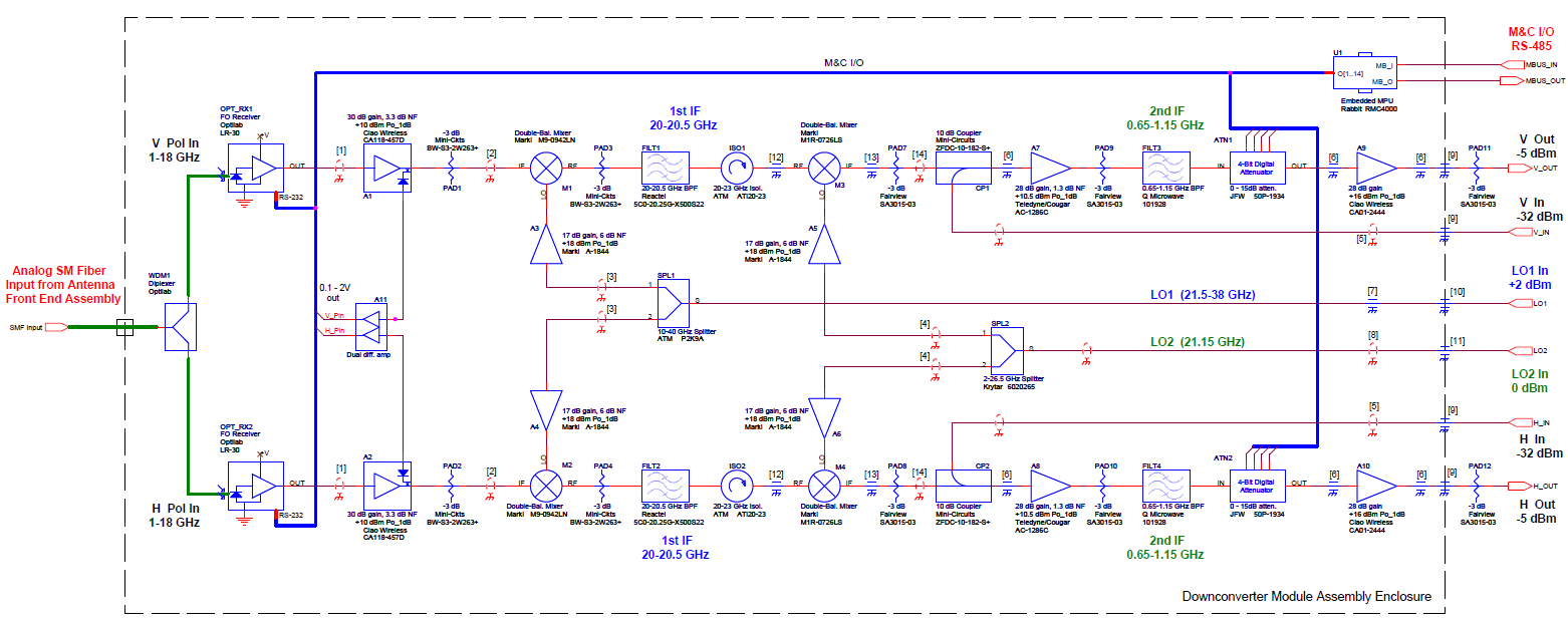
This is a dual-channel receiver, with H pol and V pol signals being received separately on optical fiber. The signals enter on the left and exit on the right. The signals are converted to electrical form, go through two stages of frequency conversion, which selects a 400 MHz intermediate frequency (IF) portion of the incoming 1-18 GHz radio frequency (RF), adjusts its power level by means of amplifiers and attenuators, and then provided this clean 400 MHz IF to the digitizers in the correlator chassis (not shown). We will discuss more about receivers and following electronics when we get to correlators.