SiMM4×4
The
SiMM4×4 Program has been developed
by Paul Rogers, Tae Dong Kang, Gelu Nita, Roman Basistyy, Michael Kotelyanskii,
and Andrei Sirenko at NJIT and Rudolph Technologies.
supported by NSF-MRI DMR-0821224 and DMR-0546985
e-mail for support and comments: sirenko@njit.edu
**********************************
To
use SiMM4×4 you need to download SiMM_1.zip or SiMM_1.rar file. SiMM4×4 can be unzipped to any folder.
The recommended location for unzipping is C:\\SiMM\ In this case
the default paths for data save/load will work from the start.
Run
Application.exe file and have fun (J).
Note:
to refresh the calculation use SPACEBAR.
Do not press ENTER every time you change input parameters, just edit the
number(s) and move the cursor away from the control field. If you press ENTER,
then the Program will try to LOAD a set of input parameters from a binary file.
Requirements:
You
need LabVIEW 2010 installed in your computer. If you have
earlier LabVIEW versions, upgrade here: https://lumen.ni.com/nicif/us/evallvuser/content.xhtml
If
you do not have LabVIEW or never used LabVIEW, just download free software:
LabVIEW
Run-Time Engine 2010
from NI website (requires
registration) : http://joule.ni.com/nidu/cds/view/p/id/2087/lang/en
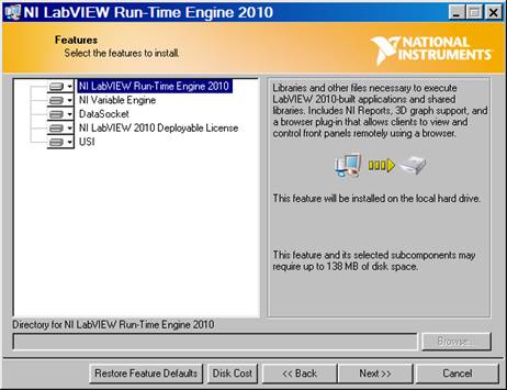
If
for some reasons (like Administrator privileges in your own computer) you have
problems installing LabVIEW Run-Time Engine 2010 in a default
configuration, try to install only the top option in the Installation Menu (see
below). Cross the other four and repeat the installation. It should work.
Theory:
The theory of light
reflection/transmission in anisotropic magneto-dielectric medium was developed
by Berreman
and was also described in the book of R. M. A. Azzam,
N. M. Bashara,
Ellipsometry and Polarized Light, North-Holland, Amsterdam, 1977. The SiMM4×4 code is based on
equations from these References. Interestingly, the SiMM4×4 code describes well
the case of the negative refractive index. Recent work of our group in this
field is published in ThinSolidFilms-2010.
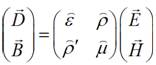
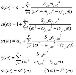
The input parameters in the model
are Eps, Mu, and Rho tensor components that connect E and H vectors
with D
and B:
In contrast to ![]() and
and ![]() tensors, the
bi-anisotropic tensors
tensors, the
bi-anisotropic tensors ![]() and
and ![]() are less known and their properties require
clarification. SiMM4×4 calculates
two major additive contributions to Rho and Rho’: the magneto-electric effect and chirality, so that:
are less known and their properties require
clarification. SiMM4×4 calculates
two major additive contributions to Rho and Rho’: the magneto-electric effect and chirality, so that:
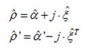
One can see
that the ME contribution is described by the complex tensor Alpha, and chirality
is represented by tensor Ksi . Both tensors, Ksi and Alpha, are complex and can have both real and imaginary parts.
Accordingly, Rho and Rho’ are not expected to
be the complex-conjugate-transpose for each other.
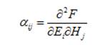
According to Dzyaloshinskii,
the corresponding ME contribution to Rho’
hould be a “transpose” tensor: Alpha’=AlphaT.
This requirement follows from the Dzyaloshinsky’s
definition of Alpha in the static
case:
Although at present this
requirement of Alpha’=AlphaT
for optical frequencies is under debate in the literature, we still use
it in the SiMM4×4 calculations. Note that both Alpha and Alpha’ have the same sign of their complex parts, so that the
oscillators in both Alpha and Alpha’ should absorb light in the
transmission experiments. Tensors Alpha and Alpha’ change sign under space
inversion and time inversion operation, remaining unchanged if both operations
are applied simultaneously. This property results in the requirement that Alpha=Alpha’
=0 in materials with the center of inversion or with time-reversal symmetry (see
Refs.[11,
12] for more detail). In contrast to Alpha, the chirality term tensor i*Ksi has its transpose-complex conjugate
counterpart -i*KsiT that contributes to Rho’. For
isotropic materials, Georgieva showed that the chirality
parameter Ksi , which originates from the time
derivatives of the electric and magnetic field vector terms in the Maxwell
equations, scales proportionally to Omega, which requires its disappearance at
zero frequency. In the case of a crystal, we assume that the chirality effect can also have a resonant behavior and should
diminish at high frequencies.
SiMM is designed for users with a general knowledge of
MM ellipsometry providing an opportunity to simulate Muller Matrix spectra in
anisotropic magneto-dielectric medium. The appropriate experimental technique
for studies of magneto-dielectric samples is full-Muller Matrix Ellipsometry.
Alternatively, one can measure Rss, Rpp, Rps, and Rsp
spectra and compare to the simulation. See recent papers by Mathias Schubert: [1] and [2].
By
request from the Community of Rotating-Analyzer-Ellipsometry (RAE), an
additional simulation option for PSI-DELTA / pseudoEps
/ n-k is included. However, for magneto-dielectric samples or anisotropic
samples with non-zero Rp, and
Rsp these simulations of
PSI/DELTA and pseudoEps / n-k can show unphysical results !!! These
simulations are added for illustration purpose only. For example, if you want
to simulate the case of a negative index of refraction in anisotropic sample,
then MM spectra behave “normally” displaying smooth variation between -1 and 1.
However, pseudo-Eps function will have unphysical
behavior (negative Eps2) in the frequency range for the negative refractive
index. So, for anisotropic samples use the option for
PSI-DELTA / pseudoEps / n-k with caution. The
meaning of the corresponding simulation is to demonstrate limitations of the
traditional RAE approach. If your simulation shows unphysical result (e.g., negative Eps2) just think about
using MM ellipsometry instead of RAE.
Manual:
The basic package covers
Reflection experiments for semi-infinite samples with Lorentz oscillator model.
In addition to that we have also developed simulations for thin films in both
Reflection and Transmission configurations, included multiple dielectric models
(Drude, coupled oscillators, etc), and
fit-to-experiment using Levenberg–Marquardt algorithm. It is available through collaboration. Send e-mail
to Andrei Sirenko: Sirenko@njit.edu
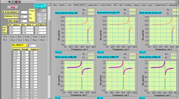
Controls are on the left, Indicators and results of simulations
are in the Tabs on the right-hand side. Control buttons are painted yellow (you can change
the values), indicators are painted blue (you can only watch
these numbers). To refresh the simulation with the new input parameter values
just press the SPACE BAR or Up/Down keys of your key-board. Omega-counts
indicator shows the progress with the calculations. The refresh rate should be
less than ~2 seconds on a modern computer for 500 data points in a spectrum. If
it takes too long, decrease the number of data points to 200.
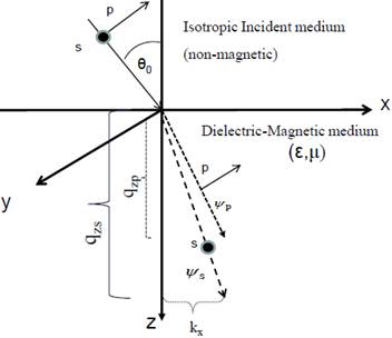
The
conventional geometry of experiment: Z is normal to the sample surface, X is in
the plane of the incidence, Y is perpendicular to the
plane of incidence.
Controls on the
left:
In
the dielectric model for Eps, Mu, and Rho tensors one can change for each of
the principle axes of the sample (X,Y,Z)
·
The
number of Lorentz oscillators, which is the same for Eps and Mu models (can be set to zero). The max number of oscillators is
< 30, the oscillator strength can be set to zero if different number of
oscillators is needed for Eps and Mu
models. For example, if you just want to simulate Eps response for Mu=1, then all Mu-oscillators should
have zero oscillator strength. The absolute values of omega's and gamma's are
taken for calculations of the tensor components:
·
Dielectric
tensor components of Eps_inf and Mu_inf accept real values only. Default
value for Eps_inf
is 10. Default value for Mu_inf is 1, but
it can be changed, of course.
·
The
default dispersion values of the off-diagonal elements of the Rho tensor are set to zero. One can add
oscillators in Rho by changing the
default oscillator strength from zero to a desired value. Note, however, that Rho2 should be less than the
product of Eps*Mu
for every frequency, but
SiMM4×4 program does not execute this limit condition (!). If you
put too much of the oscillator strength in Rho
then unphysical values will result in divergence and discontinuity of the MM
spectra. Note that Rho
diagonal components (symmetric part) is “equivalent” to an additional
contribution in Eps, while the off-diagonal part of
Rho (asymmetric part of the tensor) is “equivalent” to an additional
contribution to Mu. Reality is more
complex than this naïve explanation. Magneto-dielectric tensors are well
described in Rivera’s paper. But their Alpha
tensor is different from the Berreman’s Rho
tensor, so be careful! The Rho-prime
part is calculated automatically as shown above, so there is no control for
that part of the dielectric model.
·
The
symmetry of Eps, Mu, and Rho tensors can be different in magneto-dielectric samples.
Independent rotation of the Eps, Mu, and Rho tensors with respect to the measurements frame is
possible using the Euler’s table in the left-hand side. The default values are
all zeros that correspond to a perfect alignment of the orthorhombic sample (a,b,c axes) with respect to the
experiment reference frame (XYZ). Thus, tilt (in deg) of the sample with
respect to the experimental (s,p) reference frame (-180 --- +180 deg) can be controlled for Eps,
Mu, and Rho tensors
independently.
·
angle of incidence, AOI,:
0 - 90 deg. Normal incidence corresponds to AOI=0.
·
Ambient
refractive index can be different from 1
(default value is No=1)
TABS in the right-hand side:
|
Note |
brief
manual |
|
Eps Mu |
indicators
for the dielectric model |
|
Rho |
indicators
for the dielectric model |
|
Spectra
Eps Mu |
Spectra
for the three principle axes of Eps and Mu tensors |
|
Spectra
Rho |
Spectra
for the three diagonal and three off-diagonal components of the Rho tensor (defaults
are zeros) |
|
M,
Del, R, MM |
indicators
for the model calculations |
|
MM |
Muller
Matrix spectra |
|
Refl |
Reflectivity
spectra |
|
Psi-Delta |
Psi-Delta
spectra for RAE ellipsometry. Here you may see unphysical results for anisotropic
and magneto-electric samples |
|
Pseudo |
Pseudo
dielectric function spectra for RAE ellipsometry. Here you may see unphysical
results for anisotropic and magneto-electric samples |
|
Errors |
Errors
of the code. These fields should be empty, but for a certain unphysical input
parameter combination, there could be an error. Report them to Sirenko@njit.edu |
|
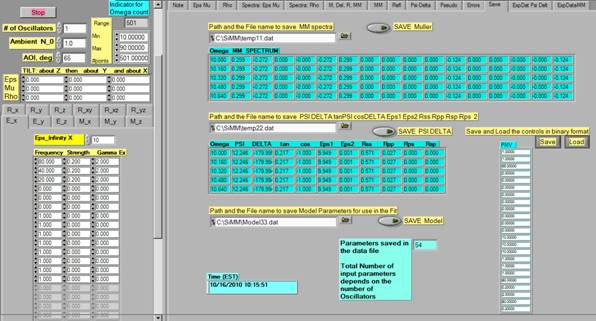
Save |
Save data of simulation for MM and for
R’s, Psi/Delta, etc. in a 2D ASCII data format that can be opened with Matlab or ORIGIN. Save data for input parameters in a
one-column format. Can be used as an input in our FITTING PROGRAM (available
through collaboration) Quick
Save / Load the set of the input
parameters in/from a binary file. Useful for quick recovery of the simulation
results. Press frequently and use different names to preserve results of your
work for different models |
|
ExpDat Psi Delt |
Here
you can open experimental data in 2D column ASCII format (or results of your
previous simulation) and compare to the results of the current simulation. To refresh the exp data alternate the
controls for the column number for the experimental file or the indicator for
the simulated function. |
|
ExpDataMM |
Here
you can open experimental data in 2D column ASCII format (or results of your
previous simulation) and compare to the results of the current simulation. To
refresh the exp data alternate the controls for the column number for the experimental
file or the indicator for the simulated function. |
Let’s start using
SiMM4×4:
Select “1” for the number of oscillators and have, correspondingly, one electric dipole at 80 cm-1 and one magnetic dipole at 60 cm-1. Press the SPACE BAR of your keyboard to refresh your simulation.
Do not press ENTER every time you change the inputs: the Program will try to LOAD a set of inputs from a binary file (e.g., Parameters1).
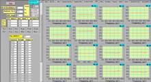
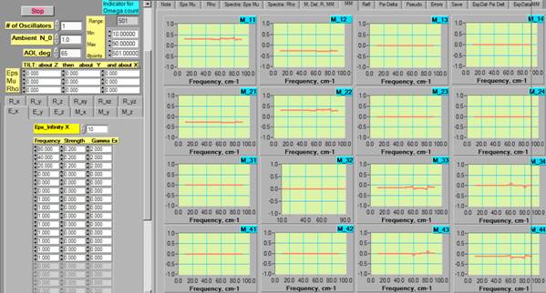
In
the MM window we will see the 16 spectra with zero off-diagonal components that
is normal for orthorhombic symmetry
Now
you can save the results of simulation and the input model parameters in this
window:
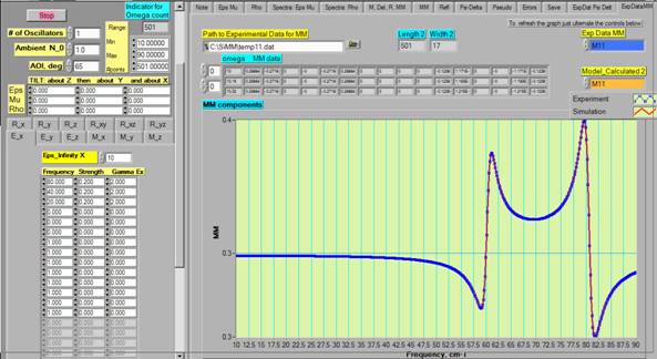
You
can “zoom” on the simulation results for each MM component in the Tab shown
below. Also, you can load your experimental data or results of the previous
simulations. The selection of the column is marked with blue. M11 corresponds
to the second column of the input data file (the first one is the “Wavenumber”, of course). The top three lines of the input
file is displayed in the window above the graph.
If
you do not see numbers that means SiMM4×4 does not recognize the format of the
input file, which should be Tab-separated multi-column ASCII with X-axis in the
left-hand side column.