%%% Exercise 1: Make a sinewave

% Fs is the sample rate.
% Most audio systems use a sample rate of 44100 Hz.
% The highest frequencies that humans can hear are typically
% in the range of 12000 to 17000 Hz. Here I chose 20 kHz.
% You can change this to see the effect of sample rate.

Fs = 20000;

% The interval intvl is the time for a single cycle at the
% sample rate. For instance, 1 Hz would be 1 second, 2 Hz
% would be 0.5 seconds, 10 Hz would be 0.1 seconds, and 20 Hz
% would be 0.05 seconds.

intvl = 1/Fs;

%% Syntax: There are three parts - a : b : c. a is the time of the first
%% sample. We can't sample at time zero - the first sample
%% will occur at a time determined by the sample rate. b is the
%% interval for every other sample starting after the first.
%% c is the final value, in seconds.

secs = 2;
tim = intvl : intvl : secs;

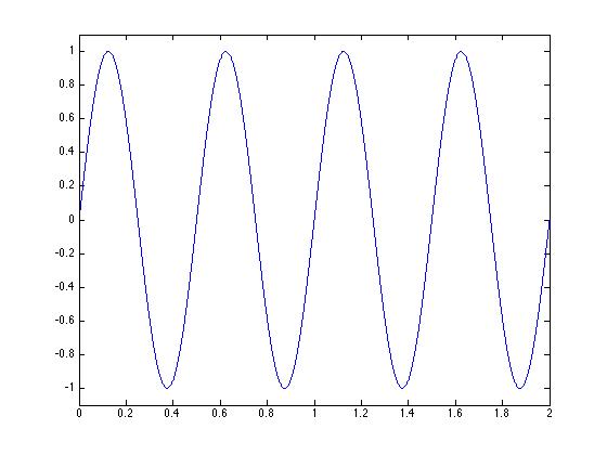
% Now we make the sinewave using the sin command. You choose
% the frequency freq - which is set
% to 2 Hz here. pi is literally the number Pi (3.1415926...).

freq = 2;
wav = sin(tim*2*pi*freq);

%-- Now we can plot. Figure A:

plot(tim, wav);

%$ EXERCISE: Learn about the role of sample rate
%$ Try changing the sample rate relative to the frequency.
%$ Here is a suggestion: Fs = 8; freq = 5;
%$ Then you can increase the sample rate to 10, 15, 20, 50, and 100.

%%% Exercise 2: Add two sinewaves

% For this exercise, the two sinewaves need to have the same duration.
% As above, we need a sample rate, and a time sequence.

Fs = 20000;
intvl = 1/Fs;
secs = 2;
tim = intvl : intvl : secs;

% We will make two signals at two different frequencies.
% Each signal can have its own amplitude - basically we can multiply
% by any value we want. Obviously, if we multiply by 0, we will get no
% signal, and 0.5, we'll get 1/2 amplitude. 1 will be the original amplitude.
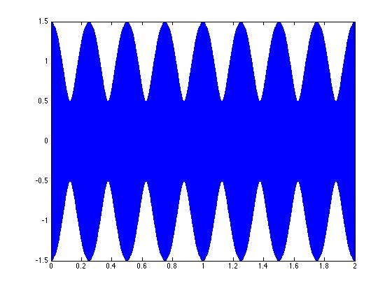
% In the example here, we have 4 Hz difference in frequencies, and the second signal
% is 1/2 the amplitude of the first.

freq1 = 1000;
freq2 = 1004;

amp1 = 1;
amp2 = 0.5;

% Make the two sinewaves

wave1 = sin(tim*2*pi*freq1) * amp1;
wave2 = sin(tim*2*pi*freq2) * amp2;

% Now add them together and plot the result

addwav = wave1 + wave2;

plot(tim, addwav);

%$ EXERCISE: Learn about interactions between sinewaves
%$ Play around by changing freq2 and amp2.
%$ Try freq2 of 1001, 1002, 1010.
%$ Try amp2 of 1, 0.1, 1.5.
%$ Plot the results using the plot command.
%$ Also plot using the sonogram command.

%%% Exercise 3: Make Sonograms - artificial signal

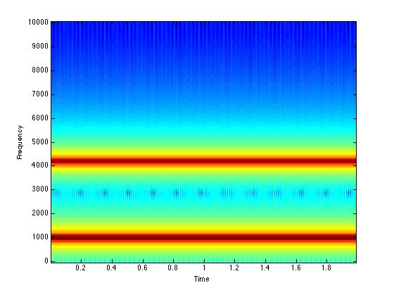
% We can make a sonogram of any signal to learn more about its spectral and
% temporal characteristics.

% We begin with the signal that we used above, except with different
% frequencies. The frequencies are further apart: freq1 = 1000 and freq2 = 4200.

Fs = 20000;
intvl = 1/Fs;
secs = 2;
tim = intvl : intvl : secs;
freq1 = 1000;
freq2 = 4200;
amp1 = 1;
amp2 = 0.5;
wave1 = sin(tim*2*pi*freq1) * amp1;
wave2 = sin(tim*2*pi*freq2) * amp2;
addwav = wave1 + wave2;

% Now we make a sonogram!
% The critical variable is 'nfft' - this is the length, in samples, over
% which the frequency will be estimate using the Fourier transform. The longer
% the length, the greater precision of the frequency estimate. nfft should always
% be a multiple of 2.

nfft = 256;
specgram(addwav, nfft, Fs);

%- specgram produces a plot

%% Bigger values for nfft lead to better frequency resolution but worse
%% time resolution. Smaller values for nfft have worse frequency
%% resolution but better temporal resolution. The artificial signal
%% we made does not change over time, so we can easily use larger values
%% for nfft.

%$ EXERCISE: Learn about the role of fft window size
%$ Try nfft = 512, 1024, 2048, and 8096 (nfft should be multiples of 2)

%%% Exercise 4: Make Sonograms - natural signal

% We can make a sonogram on any signal.

% Natural signal - we have provided two example bird songs.
% One is a White-crowned sparrow (Zonotrichia leucophrys)
% The other is a Zebra finch (Taeniopygia guttata)

% Load the wav data using the command "wavread"...
% The recording is in xxData, and the sample rate is in xxFs

Get the sound files: wcs.wav zfinch.wav

[ zfData zfFs ] = wavread('zfinch.wav');
[ wcsData wcsFs ] = wavread('wcs.wav');

% In this exercise, we will see the effect of the nfft value on the ZF song.

%% A couple of new commands: subplot and specgram...
% subplot(a, b, c); a is number of rows, b is number of columns,
% c tells which panel 1 is top left, 4 is bottom right.

% sonogram(a, b, c, d, e); a is the signal, b is the nfft, c is the
% samplerate, d and e will be explained later - e has a default
% value of 0 and does not need to be typed.

subplot(2,2,1); specgram(zfData, 32, zfFs);
subplot(2,2,2); specgram(zfData, 128, zfFs);
subplot(2,2,3); specgram(zfData, 512, zfFs);
subplot(2,2,4); specgram(zfData, 2048, zfFs);

%$ EXERCISE: Which FFT (nfft) size is best to show the details of
%$ the signal? 32, 128, 512, 2048?? You can try other values - 256 and 1024
%$ are good choices.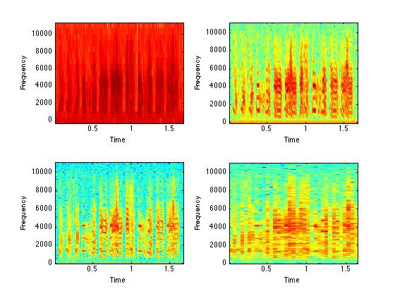

% Same for the Sparrow.

% First, make a new figure window using the "figure" command.

figure;

% Plot them!

subplot(2,2,1); specgram(wcsData, 32, wcsFs);
subplot(2,2,2); specgram(wcsData, 128, wcsFs);
subplot(2,2,3); specgram(wcsData, 512, wcsFs);
subplot(2,2,4); specgram(wcsData, 2048, wcsFs);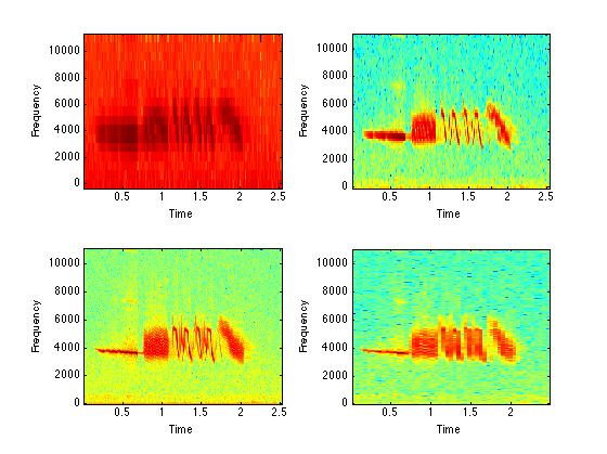

%% For short, variable signals, lower nfft values are most useful.
%% For long, constant signals, higher nfft values are most useful.
%% For wave-type weakly electric fish, which produce constant
%% frequency sinusoidal signals, we sometimes use nfft values
%% of 65536 - which provides very precise frequency resolution.

%% nfft and Fs are related.

%% If Fs is 1000 and nfft is 128, then the sample is 0.128 seconds in duration.
%% If Fs is 10000 and nfft is 128, then the sample is 0.0128 seconds in duration.
%% For the White-Crowned Sparrow, the best nfft window was 512. The song
%% was recorded at a sample rate of 22050 Hz. If the song had been recorded
%% at 44100 Hz, then the nfft window should be 1024.