%%% Exercise 5: Filter a signal

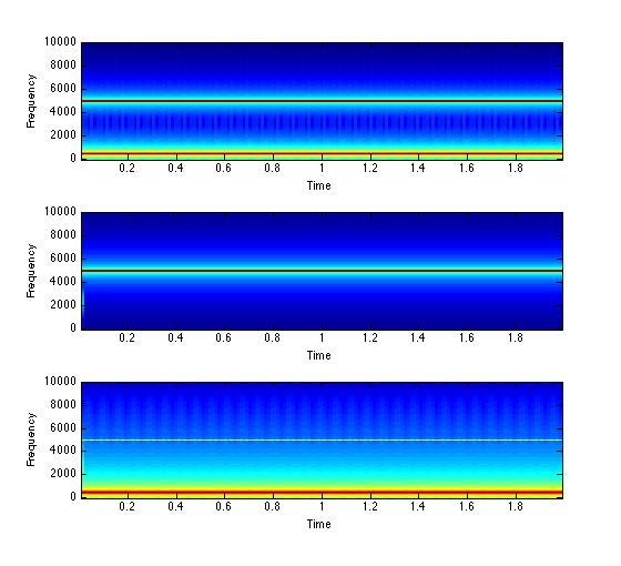
% First let's filter an artificial signal. We'll add two sinewaves together:
% one with a frequency of 5 kHz and the other at 500 Hz. We've done this before,
% so no problem!

freq1 = 5000;
freq2 = 500;

Fs = 20000;
intvl = 1/Fs;
secs = 2;
tim = intvl : intvl : secs;
amp1 = 1;
amp2 = 1;
wave1 = sin(tim*2*pi*freq1) * amp1;
wave2 = sin(tim*2*pi*freq2) * amp2;
addwav = wave1 + wave2;

% We'll do a high-pass and a low-pass filter. We can have different
% frequencies for the high- and low-pass parts, but to start we'll use
% the same frequency, 2500Hz.

lowcut = 2500;
highcut = 2500;

% These next steps make the filter. There are many types of filter -
% the one we are using is called a "Butterworth" filter. The only
% thing to change here is the 'order' - which is the slope of the
% filter. Lower numbers have a broader slope, whereas higher
% numbers have a steeper slope.

order = 5;

lowcut = lowcut*2/Fs;
highcut = highcut*2/Fs;

[b,a] = butter(order,lowcut,'low');
[d,c] = butter(order,highcut,'high');

% Here is where the filtering actually occurs. 'filtfilt' takes the
% filter that we made above, and applies it to the signal, in this case
% addwav.

lowfilt = filtfilt(b,a,addwav);
highfilt = filtfilt(d,c,addwav);

% Now let's plot the results. Top is original signal, middle is high
% pass filtered, bottom is low-pass filtered.

subplot(3,1,1); specgram(addwav, 512, Fs);
subplot(3,1,2); specgram(highfilt, 512, Fs);
subplot(3,1,3); specgram(lowfilt, 512, Fs);

%%% Exercise 6: Filter a signal - noise

% The first step is to make a noisy signal.
% Set the length, in seconds

len = 1;

% Set the SampleRate, in Hz. and make a time series...

Fs = 20000;
tim = 1/Fs:1/Fs:len;

% Make the noise sequence using randn. The arguments are in two
% dimensions… we want a 1 dimensional noisy sequence, hence the
% second dimension is '1'.

noisy=randn(length(tim),1);

% This is great - we can plot this

figure(1);
subplot(3,1,1); specgram(noisy,512,Fs);

% Now we filter, as above, and plot

order = 5;
lowcut = 1500;
highcut = 5700;

lowcut = lowcut*2/Fs;
highcut = highcut*2/Fs;

[b,a] = butter(order,lowcut,'low');
[d,c] = butter(order,highcut,'high');

% Here is where the filtering actually occurs. 'filtfilt' takes the
% filter that we made above, and applies it to the signal, in this case
% addwav.

lowfilt = filtfilt(b,a,noisy);
highfilt = filtfilt(d,c,noisy);

subplot(3,1,2); specgram(highfilt, 512, Fs);
subplot(3,1,3); specgram(lowfilt, 512, Fs);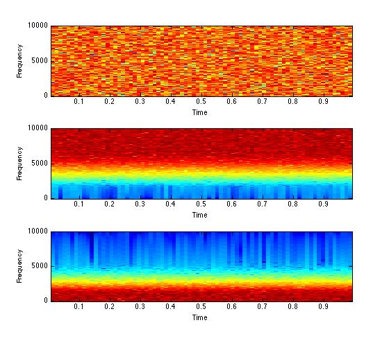

%% Now vary the 'order' of the filter between 1 and 9. What happens?

%% Can you make a bandpass signal, where you filter out signal
%% below 1000 Hz and above 7700 Hz??

%%% Exercise 7: Reverse a signal

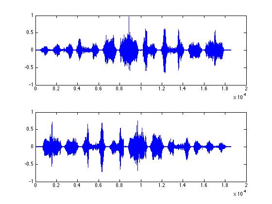
% First, we need a signal - let's use the zebra finch song

[ zfData zfFs ] = wavread('zfinch.wav');

% Now we reverse it. "end" is the last value in our variable "zfData". "1"
% is the first value in our variable "zfData". The "-1" in the middle is the
% step size. It defaults to "1" - but we can give it whatever value you want, and
% "-1" means that the steps will go 1 at a time from the end to the first value.

zfRev = zfData(end:-1:1);

% That is all there is to it...

% We can halve the sample rate for both reverse and forward songs...

zfHalfRev = zfData(end:-2:1);
zfHalfData = zfData(1:2:end);

% Let's plot!

figure(1);
subplot(2,1,1);
plot(zfHalfData);
subplot(2,1,2);
plot(zfHalfRev);

%% You can change the sample rate using this technique.

%%% Exercise 8: The "find" command

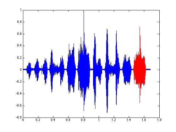
% The find command is a powerful tool to extract portions of a signal.

% First let's get a signal and plot it:

[ zfData zfFs ] = wavread('zfinch.wav');
tim = 1/zfFs:1/zfFs:length(zfData)/zfFs;

plot(tim,zfData);
% Perhaps we only want to examine the last syllable.
% We can use the "xlim" command to only plot the end.
% In this case we'll plot this syllable that starts at roughly
% 1.3 seconds and ends by 1.7 seconds.

xlim( [ 1.3 1.7 ] );

% There is also a "ylim" command for the y-axis, which does the same thing.

ylim([-0.75 0.75]);

% Now let's use the find command to get the time between 1.45 and 1.63.

pp = find ( tim > 1.45 & tim < 1.63);

% pp is now the sequence of sample positions (not samples!) for which
% tim is larger than 1.45 and smaller than 1.63.

% pp is just sequence of integers.

figure(2); plot(pp);

% But here is how we use pp...

plot( tim(pp), zfData(pp) );

% or better yet...

figure(1); plot( tim, zfData,'b');

hold on; plot( tim(pp) , zfData(pp) ,'r');

% OK - now another idea. Let's get only the values above a threshold
% Our threshold will be 0.1.

thresh = 0.1;

tt = find ( zfData > thresh );

% Now let's plot it on top of the original signal in red.
% The "hold on" command allows you to plot on the same plot again
% (the default is to erase the old plot and do the new plot).
% You can turn this off using "hold off".

figure(3);
plot(tim, zfData,'b');
hold on;
plot( tim(tt), zfData(tt) ,'r' );
hold off;