%%% Exercise 9: Separate the syllables in a song

% We need to load the data

[ zfData Fs ] = wavread('zfinch.wav');
tim = 1/Fs:1/Fs:length(zfData)/Fs;

% We are going to separate the syllables by amplitude.
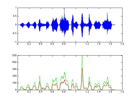
% The problem with the original signal is that it goes
% both up and down, so it is not possible to directly
% measure the amplitude. Below I describe two methods,
% "Strategy 1" and "Strategy 2", that can be used to
% make a useful measure of the amplitude.

% These two methods produce nearly the
% same result. The first method is to rectify the
% signal and low-pass filter, and the other
% is to use a function known as "Hilbert" and low-pass
% filter.

% Both require that the signal be centered at zero.
% It is easy to do this by subtracting the mean from
% the original signal.

zfData = zfData - mean(zfData);

%%% Strategy 1: Rectify and smooth

% abs is a function that takes the "absolute value"
% of the signal.

rz = abs( zfData );

% Now we are going to smooth this signal using a filter
% called "medfilt1". Here "sms" is the duration, in
% seconds, of the filter - I have set the default to
% 20 milliseconds. If sms is too long, then it will smooth
% out the signal too much. If sms is too short, then
% you will get spurious syllables.

sms = 0.020;

% we will multiply sms with the sample rate, Fs. This will
% give us the number of samples for the duration that
% sms specifies.

mrz = medfilt1 (rz, Fs*sms);

% We don't need to do the next step, but it makes life
% a little easier later. Here we multiple by 1000 so that
% the values are ~ 1 rather than 0.001.

mrz = mrz * 1000;

%%% Strategy 2: Hilbert and smooth

% This is almost identical to Strategy 1, but uses a
% nice function called Hilbert.

hz = abs( hilbert ( zfData ) );

% Now we do the same filtering as above.

sms = 0.020;
mhz = medfilt1 (hz, Fs*sms);
mhz = mhz * 1000;

%%% Plot

% The original signal

figure(1);
subplot(2,1,1); plot(tim,zfData);

% The same signal after filtering

subplot(2,1,2); plot(tim, mrz, 'r');
hold on; plot(tim, mhz, 'g'); hold off;

%%% Segment the song into individual syllables

% Animals often produce signals that are composed of multiple
% parts. One strategy to understand the signal is to divide
% it into parts. That is what we will do here - use an
% amplitude threshold to separate each part.

% Now we will replot the same data as in panel 3 of
% of Figure 1, but the y axis will be on a log scale.
% This is acheived using the plotting command "semilogy" which
% plots with the X axis normal and Y axis on a log scale. Yes,
% they also have the command "semilogx".

figure(2);
semilogy(tim, mrz);

%%%%%%%%%%%%%%%%%%%%%%%%%%%%%%%%%%%%%%%%
%
% We need to choose a threshold. We can either look at the plot
% and guess, or we can click on the plot and the computer will give
% us the coordinates where we clicked:

% First strategy - I guess "8"!

thresh = 8;

% For clicking, we use the command "ginput". The number is how many
% clicks we are going to make, which is 1 in this case.

thresh = ginput(1);

% If we used ginput, then "thresh" will have two values, % the x value and the y value of the click. We only want the y value, % which is in the second position, and hence we only want
% thresh(2). We can do the following:

thresh = thresh(2);

%%%%%%%%%%%%%%%%%%%%%%%%%%%%%%%%%%%%%%%%

% Let's replot with a line at the guessed threshold
% just to check. You might have to redo this section
% over and over again with different values for "thresh"
% until we get a value that we think will suffice.

% x will be the first and last sample of the signal.

x(1) = 1;
x(2) = length(tim);

% y will be the amplitude of the threshold

y(1) = thresh;
y(2) = thresh;

% And now we plot the line:

semilogy(tim, mrz, 'b');
hold on;
semilogy(tim(x), y, 'g');
hold off;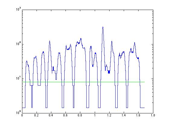

%%%%%%%%%%%%%%%%%%%%%%%%%%%%%%%%%%%%%%%%

% Now we use the 'find' command to get the part of the
% signal above the threshold. The variable "syls" will % get the index numbers for each value of mrz that is larger % than thresh:

syls = find(mrz > thresh);

% Now we're going to do something that will extract
% the starts and ends of each syllable. This seems
% complicated, but it is simple.

% Make a list of zeros that is the length of the
% signal.

zz = zeros(length(zfData), 1);

% Let's look at zz:

figure(3);

% first replot the original signal.

subplot(3,1,1);
plot(tim, zfData);

% Now plot zz... wow… zeros!

subplot(3,1,2);
plot(tim,zz,'m');

% From above, 'syls' is the list of values that are above
% the threshold - these are where the syllables are located.
% We will set zz to 1 for each of these values...

zz(syls) = 1;

% Now plot this.

hold on;
plot(tim, zz,'r');
hold off;

% Cool - these blocks roughly align with the syllables.
% But what we need are the start times and end times of
% the syllables. We will use a trick to get them...

% 'diff' takes the difference between adjacent values...
% For example sample(2) - sample(1)...

yy = diff(zz);

% Now let's plot this. Starts are marked by '1' and
% ends are marked by '-1'.

subplot(3,1,3);
plot(tim(1:end-1), yy);

% Here we use the find command to get the 'starts' and
% the 'ends'. Notice that we use "==" to indicate when we
% are ASKING if values are equal, but use "=" to SET a variable
% to a value.

starts = find( yy == 1 );
ends = find(yy == -1);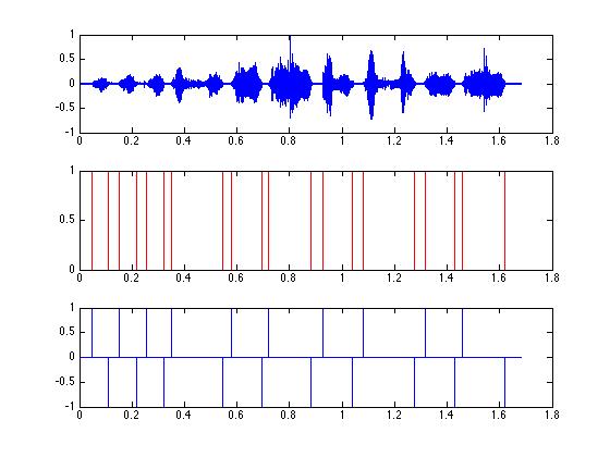

% Now this is simple! We use a loop - the 'for' command
% to get each syllable. The only part that you haven't
% seen earlier is the '{}' - called 'curly brackets'.
% syllable{1} will have the entire 1st syllable, and
% syllable{2} will have the enture 2nd syllable, etc.

% timmy and timm are not necessary, but might be useful.
% timmy is the real times from the song.
% timm is a time sequence for each syllable only.

for i = 1:length(starts)
syllable{i} = zfData(starts(i):ends(i));

timmy{i} = tim(starts(i):ends(i));
timm{i} = 1/Fs:1/Fs:(1 + ends(i) - starts(i))/Fs;

end;

% Just to show what has happened, here is a plot:
% I picked syllables 4,5,6, and 7. You can pick others
% if you wish.

figure(4);
subplot(2,4,1); specgram(syllable{4},512,Fs,[],500);
subplot(2,4,2); specgram(syllable{5},512,Fs,[],500);
subplot(2,4,3); specgram(syllable{6},512,Fs,[],500);
subplot(2,4,4); specgram(syllable{7},512,Fs,[],500);

subplot(2,4,5); plot(timm{4},syllable{4}); xlim([0 timm{4}(end)]);
subplot(2,4,6); plot(timm{5},syllable{5}); xlim([0 timm{5}(end)]);
subplot(2,4,7); plot(timm{6},syllable{6}); xlim([0 timm{6}(end)]);
subplot(2,4,8); plot(timm{7},syllable{7}); xlim([0 timm{7}(end)]);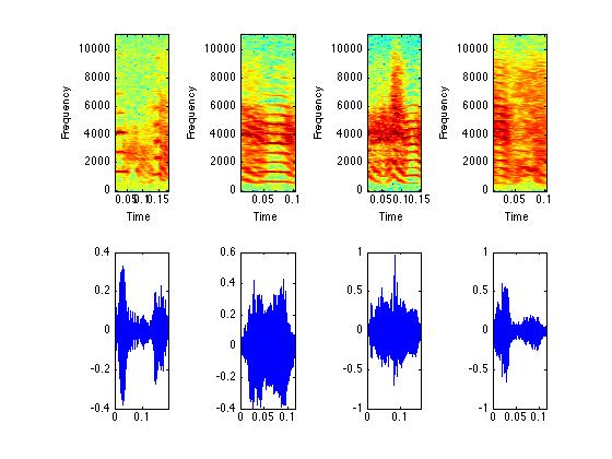

% Now we will get the silent parts between syllables.
% This can be important because sometimes the time
% between signals is an independent signal. For example,
% in frogs the duration between calls determines the
% "pulse repetition rate", which can indicate whether
% the call is a mate attraction signal or an aggressive
% signal.

% The procedure is almost the same as for the
% syllables as above. What is different is that instead
% of copying the signal from zfData, we instead make
% pure silence by putting in a flat signal with an
% amplitude of 0.

% We use a loop for each of the ends (which is the start of each silence)
% Make a list of zeros with the length of the interval
% We get the length of the interval by getting the difference
% between the end of the silence, which is the 'start' of
% the next syllable, and the start of the silence, which is
% the 'end' of the previous syllable. Complicated!?!?

for j = 2:length(ends);
nop{j} = zeros( (starts(j)-ends(j-1)), 1);

% This next step is not necessary - just a time base for the silence.

noptimmy{j} = tim(ends(j-1):starts(j));
end;

% For review: you can easily get the data for each
% syllable.
% syllable{1} is the data for the first syllable,
% and syllable{2} the second.

% Let's plot a syllable.

figure(1);
subplot(1,2,1);
specgram(syllable{7},512,Fs,512,500);
subplot(1,2,2);
plot(timmy{7},syllable{7});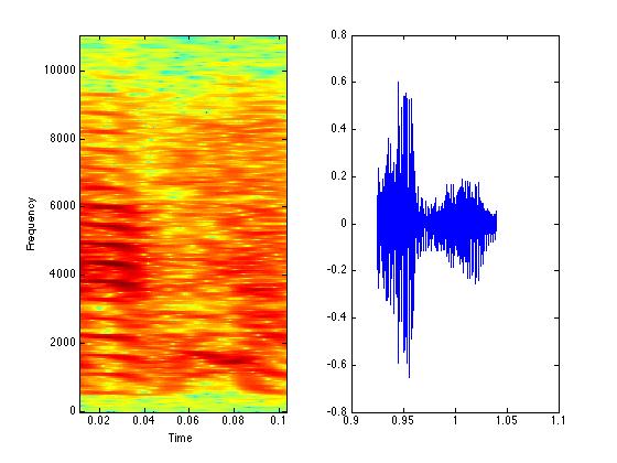

% How many syllables did we find??

length(syllable)

% How long (duration) is syllable{7}?

length(syllable{7})/Fs

%%% Exercise 10: Make a NEW song with the syllable order reversed

% Here we are making a new variable, 'revordersong' and
% we are putting the last syllable in there.
% The apostrophe - ' - changes the data from rows to columns
% or from columns to rows. In this case the data in
% 'syllable' is a column, and to concatenate them, we need
% the data to be in a row. Why this is, I don't know.

revordersong = syllable{end}';

% Now we will cycle though each syllable from the second
% to last to the first (we already have the last syllable
% from the above line.

% The variables in the brackets will be concatenated.
% so [ revordersong nop syllable ] will make
% the previously defined revordersong followed by the
% silent period, which is then followed by the next
% syllable. Recall that the apostrophe makes the
% data into a single row.

for k = length(syllable)-1:-1:1;
revordersong = [revordersong nop{k+1}' syllable{k}'];
end;

% This is nice to add - a time base for this new signal.
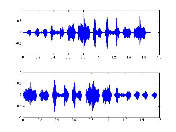
% We've seen this many times by now.

revtim = 1/Fs:1/Fs:length(revordersong)/Fs;

% now let's plot it:

subplot(2,1,1); plot(tim,zfData);

% And the reversed signal below:

subplot(2,1,2); plot(revtim, revordersong);

% or we can show the spectra...

%original signal

subplot(2,1,1); specgram(zfData,512,Fs);

% reversed signal

subplot(2,1,2); specgram(revordersong,512,Fs);

% Save the data to a wave file. You can then use
% Windows to listen to it.

wavwrite(revordersong', Fs, 16, 'revordersong.wav');

%%% Exercise 11: Make a NEW song with each syllable reversed, but the syllable order normal

% This is nearly identical to the previous exercise,
% but now the order is correct (ABCDEF) but each syllable
% is reversed.

% Take the first syllable and put it in our new variable
% revsylsong...

revsylsong = syllable{1}';

% Now reverse it - we saw how to do this in an earlier
% exercise...

revsylsong = revsylsong(end:-1:1);

% Now do the same for the rest of the syllables, adding them
% to the new variable...

% We are using a temporary variable 'ra' to do the reversing

for l = 2:length(syllable);
ra = syllable{l}';
revsylsong = [revsylsong nop{l}' ra(end:-1:1)];
end;

% and of course, the time data...

revsyltim = 1/Fs:1/Fs:length(revsylsong)/Fs;

% Cool. Now let's do the same plots...

figure(6);

% The original signal above:

subplot(2,1,1); plot(tim,zfData);

% The reversed signal below:

subplot(2,1,2); plot(revsyltim, revsylsong);

% or we can show the spectrum...

% original signal

subplot(2,1,1); specgram(zfData,512,Fs);

% reversed signal

subplot(2,1,2); specgram(revsylsong,512,Fs);

% and save to a file that we can play on the
% computer:

wavwrite(revsylsong', Fs, 16, 'revsylsong.wav');

% You can see that with these tools you can make
% a very wide range of arbitrary stimuli from
% your recordings of animal signals. These are
% powerful tools for sensory electrophysiology.

% Try to do the same exercises with the data in
% wcs.wav.

%%% Exercise 12: Spikes

% In this exercise we will take a recording of neural activity (spikes!) and
% turn them into data that we can start to analyze in useful ways.

% I have provided two sample files will nice recordings of neural activity.
% They are very different from each other.

% Read the first file, make the time data, and plot.(easy easy by now)

[a Fs] = wavread('spikes1.wav' );
tim = 1/Fs:1/Fs:length(a)/Fs;
figure(7);
plot(tim,a);

% And you can do a close up of one second of data...

xlim([3 4]);

% Now we want to set an amplitude threshold for the spikes.
% Different recordings will have different amplitudes
% for spikes.
% Here I have guessed that 0.5 will be sufficient. Look
% at the plot to confirm.

thresh = 0.5;

% We use the find command to get all of
% the data above threshold.

spikes = find( a > thresh );

% This is a complicated, but necessary step. Spikes are
% more than 1 or two milliseconds in duration. Thus, we
% want a threshold
% for the interval between spikes - anything less than
% that threshold is a mistake from the find command.

% Our threshold will be 1 millisecond: 0.001 seconds.
% Since are data is in samples and not in milliseconds, we'll
% set our threshold to the sample rate * milliseconds.

% 'diff' is the difference between adjacent data points.
% So, here we find all of the instances where the number of
% samples between spikes is greater than our threshold of
% 1 millisecond samples (which for Fs = 10000 is 10 samples).

spikes1 = spikes( find( diff(spikes) > 0.001*Fs));

% How many spikes did we find?

length(spikes1)

% What is the spike rate??

length(spikes1) / tim(end)

% Now let's plot. We'll plot a STAR at each time
% that a spike occurred. The 'ones' command is
% identical to the zeros command, except that each
% value is one. This would be OK, but I decided to
% multiply it by the threshold so that the dots
% will be at the level of the threshold when we
% plot it. you will see...

ys = ones(length(spikes1),1) * thresh;

% Now plot...

plot(tim,a,'b');
% Markersize changes the size of the symbols.

% Try the same plot with 1 or 3 or 4 to see
% what happens to the plot.

hold on; plot(tim(spikes1),ys,'r*','markersize', 2);
hold off;

% Now zoom in!

xlim([1 2]);

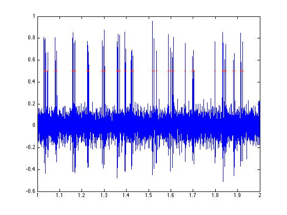
% even further...

xlim([1 1.25]);

% Another important measure is the time between spikes
% This is very easy to get using the 'diff' command.
% diff will give use the number of samples between
% spikes, and then we divide by the sample rate to
% get the time, in seconds, between spikes.

intervals1 = diff(spikes1)/Fs;

% Here are some easy measurements...

mean(intervals1)
max(intervals1)
min(intervals1)

% But looking at the plot, we see that the spikes
% are in "bursts" rather than randomly spread.
% If they were randomly timed, we would find a
% random distribution of the intervals between
% spikes. Let's take a look using a histogram...

hist(intervals1,100);

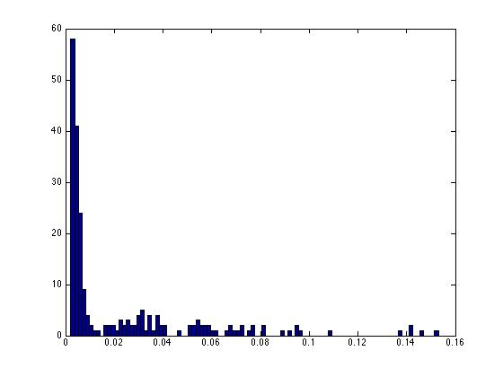
% For these data we see that there are many many
% intervals below 0.015 (15 milliseconds), and a
% spread of longer intervals.
% This plot is a very good example of a "bursty" neuron.

% The other data, spikes2.wav, is very very different.

% Please do the same analysis for those data as you
% did for spikes1.wav. Use different variable names
% like changing spikes1 to spikes2 and interval1 to
% interval2. so that you can make the following plots...

% Data from spikes1,wav
subplot(2,1,1);
hist(intervals1,100);

% Data from spikes2.wav
subplot(2,1,2)
hist(intervals2,100);