IDL Tutorial

In association with Lab #3 of Phys 322, Observational Astronomy

Start IDL:

To start IDL, click on the “checkerboard” icon on the left in the task bar. After a moment, a window will appear with a blank gray area on the top, a white area in the bottom half of the screen (the log window) where text output will appear, and a line along the very bottom where commands can be typed.

Open a blank display window:

To open a blank window, simply type

window

at the command prompt (the command entry line at the bottom). You should see a black window in the upper-right quarter of the screen with the title IDL 0. This is where plot or image output will go.

Read in an image:

We have an image of Saturn on the disk, taken at the Boyden Hall observatory. It is in a format called FITS (Flexible Image Transfer System), which is commonly used in astronomy. Type in the following command to read the image using the readfits procedure:

satraw = readfits(‘c:\working\images\saturn.fit’)

where the argument is just the filename and path to the file saturn.fit, located in the c:\working\images directory. The variable name satraw will be used to refer to the image, and we can think of it as containing the image.

Display the image:

To display the image, type the command:

tvscl,satraw

You should see a gray-scale image of Saturn in the right-hand side of the display window. The command tvscl does two things—it scales the values in the image so that they cover the full 8-bit range of the display, but no more, and then it transfers the values to the TV device (the display window) for display. Note: if you do not see the display window, it may be behind the command entry window. You can bring the display window to the front by typing the command:

wshow ; Window-show, brings the display window to front.

Use the cursor routine to find the location of Saturn:

Type the command

cursor,x,y,/dev ; Read the device coordinates of the cursor.

which waits until the user clicks the mouse on the display window, then puts the device coordinates of the mouse pointer into the variables x and y. After typing the command, move the mouse to center on Saturn and click the left mouse button. To see what the coordinates are, use the command

print,x,y ; Print the variables x and y to the log window.

You should see something like this in the log window

IDL> print,x,y

444 196

These are the pixel numbers of the center of Saturn in the image.

Extract a small portion of the image around Saturn:

You can refer to parts of an image (horizontal and vertical ranges of pixels) by using the range expression: min:max, so that 0:10 would refer to 11 pixel range from 0 to 10. We want to clip out a 40 by 40 pixel area around the position returned by the cursor command and put it into a new variable called saturn. We use the following command to do this:

saturn = satraw[x-19:x+20,y-19:y+20]

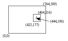which you should be able to understand as taking a range from columns 425:464 in the x direction and rows 177:216 in the y direction. The geometry of the situation is shown in the figure at the right. To verify that the small sub-image is 40 pixels by 40 pixels, use the help command, which just prints the size of arrays. For example

help,saturn

prints the following to the log window

SATURN UINT = Array[40, 40]

indicating that the variable saturn is an unsigned integer array of size 40 x 40 pixels.

Display the small image:

To display the small image represented by the variable saturn, just use the tvscl command as before:

tvscl,saturn

which this time will show the smaller image in the lower-left corner of the display window. Notice that the rest of the display window is unchanged, and still has the larger picture showing. You can use the erase command (no arguments) to erase the display if you wish.

Print the contents of the variable saturn:

To demonstrate that images are just arrays of numbers, print out the values in the variable saturn by typing the command

print,saturn

which will fill the log window with a lot of numbers (40² = 1600 numbers). You may notice that the numbers range from a low of about 100 up to about 5000. To find out the true range of numbers, we can use the max and min commands. The comand

print,min(saturn),max(saturn)

prints

117 6200

We can display the image in numbers, and fit it all one the screen, if we scale the numbers to range from 0 to 10. The following command does this:

print,fix(10.*saturn/max(saturn)),format='(40i2)'

You should be able to see the image of Saturn in the numbers printed to the log window. To understand this command, note that saturn/max(saturn) scales the numbers from 0 to 1, so we multiply these numbers by 10 to scale from 0 to 10. The fix function just converts these real numbers to integers. The format string, ‘(40i2)’, tells the print command to print a row of 40 numbers with each number taking 2 spaces.

Display the image of Saturn in different ways

Once we have an image contained in a variable, IDL can display it in a nearly infinite number of ways. Try each of the commands below:

tvscl,congrid(saturn,200,200) ; stretch the image to 200 x 200

tvscl,congrid(saturn,200,200,/interp) ; stretch with interpolation

loadct,3 ; change color table to red

tvscl,congrid(saturn,200,200,/interp) ; and redisplay

loadct,39 ; change color table to rainbow

tvscl,congrid(saturn,200,200,/interp) ; and redisplay

shade_surf,saturn ; display as a 3-d surface plot

Print a color photo of Saturn

To send an image to the printer, you must change the plot device to the printer, send the image to the new plot device, and close the plot device (which ejects the paper). Do not forget to change the plot device back to the default one (the screen), which is referred to as ‘win’. The following commands do this for the enlarged rainbow image of Saturn:

set_plot,’printer’ ; set the plot device to printer

tvscl,congrid(saturn,200,200,/interp) ; send the image to the “tv”

device,/close ; close the plot device

set_plot,’win’ ; reset the device to “windows”

A quick look at noise

Reset the display to gray color table and redisplay the satraw image:

loadct,0 ; change color table to gray

erase ; Erase the display

tvscl,satraw ; Redisplay the satraw image

Although the background appears completely black, this is only because the brightest parts of the image are being scaled to the maximum of the display, which is a level of 256 (2⁸ or 8-bit). We can see the noise level in the image by clipping the image to a level just above the noise, say a value of 150, as follows:

tvscl,satraw<150 ; display satraw, but clip to 150

Suddenly we can see the noisy background, and we can even see at least two moons of Saturn.

Let’s take a closer look at the noise. Clip out the bottom section of the satraw image (the first 50 rows of the image) into a new image called noise:

noise = satraw[*,0:49] ; clip out the bottom 50 rows of satraw

where we have used a short-cut—the ‘*’ stands for the entire x range of the image, and is the same as if we had typed noise = satraw[0:764,0:49]. Let’s plot a single row of the noise image:

plot,noise[*,0] ; plot the bottom row of the image

The plot command just plots the array of numbers as a line plot, but we can think of it as a cut across the image. You can see how noisy the background is. Try plotting some other rows by changing the zero to other numbers.

A quantitative look at the noise

We can think of the noise as a background light level of about 120, plus random fluctuations from pixel to pixel of the CCD camera that add or subtract from the background. How “noisy” is it? We can quantify the noise by using the moment function as follows:

print,moment(noise) ; print the mean, variance, skew and kurtosis

which results in four numbers being printed to the screen,

119.706 36.0322 0.0836252 0.907063

The first number, about 120, is the mean value over the entire image. The second number is the variance, and the square-root of the variance is called the standard deviation, . This means that if the noise is distributed according to gaussian statistics, there is about a 63% chance that a particular value will be within s = 6 units of the mean, a better than 95% chance that it will be within 2s = 12 units of the mean, and a better than 99% probability that it will be within 3s = 18 units.

We can reduce the noise by averaging. For example, we can average all of the rows of the noise image into a single average row (which we will name average) by using the total function:

average = total(noise,2)/50. ; Sum the second dimension of noise

which sums the second dimension (the rows) of the noise array and divides by the number of rows (50) to obtain the average of the rows. Let’s overplot this onto our previous plot:

oplot,average,color=150 ; overplot, using color value 150

You should see a light gray line plotted over the previous plot, which clearly has greatly reduced noise. If we average 50 numbers, the standard deviation should drop by a factor of =7.1, to 6 / 7.1 = 0.84, but if we apply the moment function to our average array

print,moment(average)

we find a standard deviation of about 3.5. That is because the background is not flat, but rather has a slope, gently increasing from left to right. This skews our measurement of the noise. To get a valid noise measurement, we should “flatten” the image to remove these slow variations across the image. We will learn more about flattening later.

Final comments

This tutorial has introduced some of the more useful commands in IDL, although there are many more that we could use, and the commands that we did use have other features that we have not explored. To learn more about a command, use the on-line help by selecting Contents… from the Help menu, select the Index tab, and type in the name of the command.

In this tutorial you should have learned that images are just arrays of numbers, and mathematical manipulations are used to correct for different unwanted effects, as well as bringing out details that may not be apparent in the raw image (like the presence of the two moons of Saturn). We will be using IDL to explore and analyze images for scientific measurements, as well as improving the images for aesthetic appeal.

Please feel free to explore IDL with the Saturn image or others, and indulge your curiosity.