Physics 728
Radio Astronomy:  Lecture #3
Prof. Dale E. Gary
NJIT

Radiative Transfer

Propagation of Radiation

We have discussed the generation of radiation by considering the volume emissivity, ην, which is the energy per unit time per unit volume per unit frequency bandwidth per sterradian.  Note that these units are the same as intensity, except it is per unit volume instead of per unit area.  We will now discuss the total emission along a raypath through the plasma (loosely the same as the line of sight).
Along the raypath, more photons are added from each volume element, but also photons generated in one volume element can be absorbed in the same or another volume element.  The increment in intensity, dI, in a volume element can be written as
dI = ην dl − κνIdl,        (1)
        source    sink
        term      term
where we introduce the absorption coefficient, or opacity, κν, which is the fraction of intensity I absorbed per unit length.

In thermodynamic equilibrium, Kirchoff's law states that emission and absorption occur at the same rate (the principle of detailed-balance).  If this were not true--say absorption were greater than emission--then the gas would heat up and would no longer be in thermodynamic equilibrium.  If emission were greater than absorption, the gas would cool.  In either case, ultimately the gas would come back into equilibrium such that emission exactly balances absorption.  In this special case, of course, dI = 0, and I = Bν(T), the Planck function, so in the Rayleigh-Jeans limit equation (1) implies that

Bν(T) = ηνν = 2kTeν2/c2.        (2)
We will come back to this relationship between emissivity and absorption coefficient in a moment.
External Absorption
Consider a cool cloud with a hot source of radiation behind it.  The radiation will enter the cloud with intensity Io, but will be absorbed on passing through the cloud.
In this case, we are assuming that the cloud itself provides negligible emissivity, so equation (1) becomes
dI = −κνIdl,
where I is the intensity entering each volume element.  This is a trivial differential equation whose solution is
    L
I = Ioexp(
κν dl).
 
  0
 

Note that the integration is taken along the line of sight from the observer.  In the case where the absorption is constant, of course, κν can be brought out of the integral.  The integral quantity is a dimensionless quantity called the optical depth, and designated τν.  Using this notation, the intensity exiting the cloud is just

I = Ioe−τ
The optical depth is a convenient way to refer to the "thickness" of a cloud.  It basically measures how many e-foldings of intensity reduction the cloud's thickness represents.  A cloud with τν >> 1 is said to be optically thick, while a cloud with τν << 1 is optically thin.  Optical depth unity is thus an important dividing point between regimes.
Equation of Radiative Transfer
We can rearrange equation (1) to give a first-order ordinary differential equation (the equation of radiative transfer) for I, i.e.
dI/dl + κνI = ην .           (3)

Such a differential equation can be solved by use of an integrating factor, so let us remind ourselves of that approach:

The above equation is of the form y' + p(x) y = q(x), where y = I, x = l, p(x) = κν, and q(x) = ην. Here we are using the notation y' = dy/dx = dI/dl. To obtain the integrating factor m(x), multiply through by m(x) and seek a solution [m(x)y]' = m(x)q(x), that is:

m(x)y' + m(x)p(x)y = m(x)q(x)

and

m(x)y' + m(x)' y = m(x)q(x)

from which we identify m(x)' = m(x)p(x). The solution to this gives the integrating factor m(x) = ep(x)dx = eκν dl. Using this integrating factor, we can solve the easier equation [m(x)y]' = m(x)q(x), i.e.

m(x)q(x)dx.
y =
  ___________________
 
m(x)

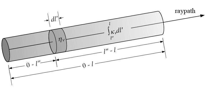
We want to use this form to solve the equation, but in order to do so we have to be very clear about the geometry this applies to. Below is the new geometry we are now interested in. We are considering an emitting element as before, but it is located at l'', somewhere along the path from 0 to l, and we will integrate over all emitting elements of length dl' from 0 to l. The key thing to notice is that emission from the element at l'' will only be absorbed over the remaining length, from l'' to l.

Substituting the values for x, y, m(x), q(x) in the above equation, we have the differential equation we wish to solve:

.

It is at the point of integrating both sides with respect to l that we have to introduce the "dummy" integration variable l'' on the right-hand side, which corresponds to the location of our volume element as in the above figure.

.

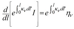
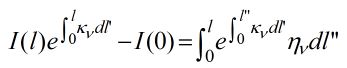
We now isolate I(l) on the left to get:

.

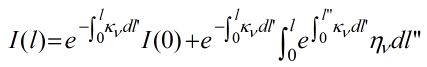
Note that the exponential outside the integral over dl'' is a constant--it is just a numerical factor. Hence, it can be moved inside the integral for an important simplification:

.

The interpretation of the integral quantity is that the emission from an element at position dl'' along the raypath is absorbed by the overlying material, i.e. there is extinction of the emission found by integrating the absorption coefficient from l'' to l, the top of the column. Finally, we can use the concept of optical depth we introduced earlier, which is formally just a change of variable:

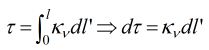
When we do this, the limits of the integration, originally from 0 to l, go from τ to 0, because optical depth is defined, as the name implies, as a depth from 0, where we are, to the depth of the source.

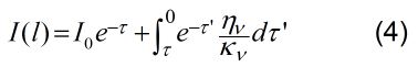
It is very useful to look at this equation in the case of a homogeneous source, i.e. one for which both the emissivity and absorption coefficient are constant along the ray path. In that case, ην and κν can be taken out of the integral, and we obtain:

I = Ioe−τ + ηνν(1− e−τ).        (5 -- homogeneous source)
Note that the first term is just the same solution we got in the previous section, and represents the contribution of an external source along the line of sight.  The second term represents the contribution from the internal emission and absorption of the cloud.  Now we come to a nice simplification that we can use in the Rayleigh-Jeans approximation. We write I = 2kTbν2/c2, Io = 2kToν2/c2, and from equation (2), ηνν = 2kTeν2/c2 to obtain:
Tb = Toe−τ + Te(1− e−τ),        (6 -- thermal source)
where Tb is the brightness temperature that we introduced in the first lecture, we have characterized the intensity of the external source in terms of an equivalent temperature To , and we have used equation (2) to relate the ratio of emissivity to absorption coefficient as the Planck function.  We have essentially divided equation (5) by 22/c2.  The use of equation (2), of course, assumes thermodynamic equilibrium, so it only holds for a thermal source.  However, equation (6) still holds for homogeneous nonthermal sources so long as we replace Te with Teff = E/k :

ην/kν = 2kTeffν2/c2.                    (2')


Tb = Toe−τ + Teff(1− e−τ).        (6' -- nonthermal source)

There is one additional approximation that is very useful.  Recall the two regimes of optical depth, τν >> 1 (optically thick), and τν << 1 (optically thin).  In these two regimes, equation (6') becomes:
Tb = Teff,                            τν >> 1 (optically thick regime)          (7a)
Tb = To(1−τ) + Teffτ.        τν << 1 (optically thin regime)            (7b)

In many cases, it is convenient to think about a given situation in terms of equations (7), although one should keep in mind the form of the more correct equations (6 and 6').

One more reminder, equations (5), (6) and (7) all assume a homogeneous source. It is very common and useful when thinking about radiative transfer to consider plane parallel atmospheres, i.e. a stack of homogeneous slices of atmosphere (usually limited to one or two!) that represent the "equivalent" situation. However, when one actually wants to model a true situation where inhomogeneity is important, it is necessary to go back to equation (4), which contains no approximations. To do that, one obviously needs to know both ην and κν separately, so that is what we will explore next.

Opacity of Emission Mechanisms
In the previous lecture we wrote down some expressions for emissivity for certain emission mechanisms.  However, in radio astronomy it is often simpler to use equations (6) or (7), which require the opacity of a given mechanism, instead of the emissivity.  Note that equation (2') shows that these are quite simply related, and in fact I wrote down the emissivities in the previous lecture from expressions for opacity that I found in the literature, by converting from opacity to emissivity using equation (2').

We are now in a position to understand the radio spectrum due to various emission mechanisms by considering the expression for opacity for each mechanism, and the equations (7).

Thermal Bremsstrahlung
Let's start with thermal bremsstrahlung (free-free emission).  The emissivity was given in Lecture 2 as:

ην = (26πe6/3mec3)(2π/3mekT)1/2 neniZ2 Gff(T,ν).
which we noted was independent of frequency except for a slight frequency dependence of the Gaunt factor Gff(T,ν).  Using (2), we have
κν = (1/3c)(2π/3)1/2p/ν)2[4πneΣ(niZi2)e4/me1/2(kT)3/2]Gff(T,ν)
     = 9.78 x 10⁻³neΣ(niZi2)/(ν2T3/2)                                                                 (8)
x { 18.2 + ln T3/2 − ln ν     (T < 2 x 10⁵ K) 
24.5 + ln T − ln ν        (T > 2 x 10⁵ K)
where two values for the Gaunt factor are given for conditions of the solar atmosphere.  Note that the optical depth goes as ν−2, so is greater at lower frequencies.

The complete spectrum, for conditions of the solar corona (T = 106 K, fully ionized hydrogen + 10% helium) will be found by inserting (8) into (6), assuming τ =κ dl = κ L, where L is the relevant length of the line of sight through the corona, typically taken to be the density scale height L = 0.1 Rsun. The figure below plots the brightness temperature spectrum, assuming that the corona overlies a 10,000 K, optically thick chromosphere.


Thermal Bremsstrahlung brightness temperature spectrum for an iso-thermal
solar corona at 106 K, plus a 10,000 K chromosphere.  The dashed line shows
the result without a chromosphere.

This is the brightness temperature spectrum.  The flux density spectrum is obtained from equation (5) of Lecture 1, where the brightness is integrated over the source size or the beam size, whichever is smaller.

Gyroresonance Emission
In Lecture 2 we gave the emissivity for thermal gyroresonance emission.  Here is the corresponding expression for opacity:

κν(s,θ) = π2/4cσd(ωμσ/dω]−1p2/ν)(s2/s!) [s2β2sin2θ /2]s−1[βcos θ]−1
                x exp[−(1 − sνB/ν)2/(2 μσ2β2cos2θ)](1 − σ|cos θ|)2             (9)
where σ = +1 for o-mode (circular polarization in which the electric vector rotates in the direction opposite the direction of the spiraling electrons, and σ = −1 for x-mode (circular polarization in which the electric vector rotates in the same direction as the electrons), and μσ is the index of refraction for the mode.  To use this with equation (6), one must multiply by an appropriate scale length.  For the case of gyroresonance emission, the scale length is derived from the narrowness of the resonance around sνB, given by the exponential "line-shape" term in (9).  An appropriate scale length is L = 2LBβcos θ, where LB = B/grad(B) is the scale length of the magnetic field.  Note that to determine the overall opacity, one calculates (9) separately for s = 1, 2, 3..., and then adds the contributions to get an overall opacity.  A numerical calculation, given an atmospheric structure of ne, Te, B, and θ as a function of position along the line of sight is straightforward.

Thermal gyroresonance brightness temperature spectrum for an iso-thermal
solar corona at 106 K, plus a 10,000 K chromosphere.  The line spectrum is
what we would see if the magnetic field were uniform at 500 G.  The smooth
spectrum shown by the heavy line is that expected in the more physical case
of a smoothly varying magnetic field, with maximum field strength 500 G.

Gyrosynchrotron Emission
Recall that gyrosynchrotron emission is the same basic mechanism as gyroresonance, but for higher-energy electrons, and so the emission occurs at higher harmonics, typically in the range s = 5-100.  These electrons may have a "super-hot" thermal distribution, or a power-law energy distribution, or any other physical distribution.  Analytical expressions for the thermal case are possible but extremely complicated (see Dulk, 1985, pg 179).  Analytical expressions for the power-law case are not possible, but numerical calculations show that the dependence of the emissivity and absorption coefficient are sufficiently simple over some parameter ranges that empirical expressions can be given.

Here are the plots of emissivity, opacity, effective temperature (ratio of emissivity to opacity), and degree of polarization (top four panels), for a power-law distribution:


From Dulk (1985), Ann. Rev. Astronomy & Astrophysics, 23, 169.  Solid lines are for q = 40o, while dashed lines
are for q = 80o.  The top four panels are for powerlaw electron distributions, while the bottom two panels are for
a thermal distribution of electrons.

Note that these log-log plots show some curvature at low harmonics, but above about s=10 they are nearly straight lines (i.e. power-laws) in the various parameters.  By fitting power-law functions to them, the following empirical equations were derived that give reasonably accurate results in the range s = 10-100:

The plot of Teff shows the optically thick spectral shape, while the plot of ην shows the optically thin spectral shape.  I want to show how the spectral shape varies as the number of particles changes, which I will do interactively in Photoshop...  Note that both ην and κν are scaled by the number density, N, of radiating electrons, which makes sense.  They are also shown scaled oppositely with respect to B, but I am not sure of the reason.
More on Propagation
At the beginning of this lecture we noted that we were considering propagation along a raypath.  What do we mean by that?  As the e-m waves propagate, they can refract due to the changing index of refraction in the plasma.  We need to derive the general formula for the index of refraction.  We have also mentioned several times that electromagnetic radiation can be in the x-mode or o-mode, which are two modes of opposite circular polarization.  It is time to introduce something about that.  A full treatment is well beyond the scope of this lecture, so I just want to introduce the subject and write down the full expressions for propagation of these two modes in a plasma.

Consider a geometry with propagation of an e-m wave (k direction) at some angle θ from the magnetic field, and define the plane containing k and B as the x-y plane.  The part of B along k we will call BL, and the part transverse to k we will call BT.  We can write down the equations of motion for electrons under the Lorentz force, and we can introduce the influence of collisions by considering a collision frequency νc, and write the average force (average rate of loss of momentum) as mvνc.  Writing time derivatives with primes (e.g. ax = x'' and vx = x'), the three equations of motion for different components are:

mx'' = eEx− ez'BT/c − mx'νc
my'' = eEy − ez'BL/c − my'νc
mz'' = eEz + ex'BT/c − ey'BL/c − mz'νc
We then seek wave solutions to this set of coupled equations using the fourier method, and write the resulting equations in terms of the volume polarization, e.g. P = neex.  The solution is a bit complicated, and makes use of some relations that we would have to take time to develop, but the end result is the Appleton formula, which is the index of refraction in a plasma, written in terms of ratios of frequencies:
X = ωp2/ω2 ;
Y = ωB/ω;
Z = νc/ω;
where ωp2 is the plasma frequency that we mentioned earlier, ΩB is the gyrofrequency, and νc is the collision frequency.  The index of refraction is:
 
X
n2 = 1 −
   (Appleton formula)
1 − iZYT2/2(1 − X iZ) + σ[YT4/4(1 − X iZ)2 + YL2]1/2 
where σ = +1 for o-mode and σ = −1 for x-mode (as before when we gave the expression for gyroresonance opacity).  Here, YL and YT  are the longitudinal and transverse parts Y, and involve the gyrofrequency for the corresponding components of BL and BT.  When we can ignore collisions (Z = 0), the index of refraction becomes purely real and we have:
2X(1 − X)
μ2 = 1 −
   (Appleton-Hartree formula)
2(1 − X) − YT2 + σ[YT4 + 4(1 − X)2YL2]1/2 

Let's look at some results of this formula:

No magnetic field and no collisions
In this case, the index of refraction becomes very simple:

μ2 = 1 − X = 1 − ωp2/ω2
In most mediums you may be familiar with, you are used to the index of refraction being greater than one, but for a plasma (with no magnetic field) the index of refraction is always less than 1.  Since the index of refraction is the ratio of speed of light in a vacuum to phase speed in the medium, this means that the phase speed in the medium exceeds the speed of light!  But the group speed is less than the speed of light, so it does not violate special relativity.  Note what happens when ω < ωp.  In this case, the index of refraction becomes imaginary (μ2 < 0), and the e-m wave is evanescent (cannot propagate).  So there is a limit to how low a frequency the plasma can support, and waves at frequencies below the plasma frequency cannot propagate (see the figure below).

Notice that the emission from this type III burst, which is due to plasma emission at the
local plasma frequency, stops abrubtly at about 7 kHz.  That is because the Ulysses
spacecraft is embedded in plasma whose plasma frequency is 7 kHz, so radio waves
at frequencies less than this cannot reach the spacecraft.  You can determine the local
electron density from this fact.

As another example, if one sends a radio wave from the ground, vertically through the Earth's ionosphere, it will propagate upward initially with μ2 = 1, but as it enters the ionized medium (the plasma) μ will become smaller as the density increases (as ωp increases).  If the frequency of the wave is high enough (above about 8 MHz), μ will never reach zero, so although the group speed slows down (the signal is delayed), it still makes it through.  However, if the frequency is below 8 MHz, the wave will propagate only until μ = 0, at which point it will reflect and propagate downward.  This is why shortwave radio signals skip off the ionosphere.  If the propagation is not vertical, but is instead at some angle φo from the ground, then the reflection will occur earlier, when Snell's Law, μ sin φ = μo sin φo is satisfied for φ = 90.  Thus, the reflection will occur at a value <&mul = sin φo.  So for radio waves propagating at some angle, the reflection will occur even at higher frequencies, up to 25 MHz or more.  The ionosphere and the ground form a kind of waveguide for shortwave communication.  It is worthwhile in this context to mention that when collisions are important, the radiation can be absorbed (due to imaginary part of μ2).  This occurs when solar X-rays ionize the lower atmosphere of Earth (the ionosphere, normally collisionless, extends to lower heights of higher density), and can cause loss of shortwave communication (so-called shortwave fadeout).

Magnetic field, no collisions
In this case, the plasma becomes birefringent, that is, there are two distinct modes in the plasma, again called the o-mode and the x-mode.  Let's see where the index of refraction reaches zero (that is, where the waves become evanescent, or reflect):

X = 1              (o-mode)
X = 1 − Y        (x-mode, valid for Y < 1)
X = 1 + Y        (x-mode, valid for Y > 1)
The top two expressions are the reason that plasma emission tends to be o-mode polarized in the solar corona.  Plasma emission, by its very nature, is generated near the plasma frequency, which is allowed for o-mode, since there μ = 0, but is not imaginary.  For x-mode, however, the second expression X = 1 − Y says that frequencies ω < ωp + ΩB/2 will be evanescent.  Since the plasma emission is generated at ω = ωp, this condition is fulfilled, and the x-mode is evanescent and thus not produced.  There is a thermal width to the plasma frequency resonance, however, so in some cases some x-mode emission can escape, but only for small B.

In the example of reflection from the Earth's ionosphere, one must take into account the Earth's magnetic field.  As a consequence, for normal propagation, o-mode polarized radiation will reflect at the layer where X = 1, (i.e. ω = ωp, as before), but x-mode radiation will reflect at a lower layer, where X = 1 − Y.

Overview of the Emission and Propagation Process
To put all of this together, we have the following processes:
  • emission from single, charged particles occurs typically due to accelerations by various forces, although any process that leads to transverse electric fields will lead to radiation.
    • electrons are far more efficient than ions for radiation
    • radiation process is defined by the cause of the accelerations
    • more than one radiation process can be active at once
  • to determine the emissivity for a radiation process, one must integrate over a distribution of particles
    • thermal emission
    • nonthermal emission => powerlaw distribution or other, more complex distributions
  • the radiation propagates through the plasma
    • may refract due to changing index of refraction
    • intensity increases along the raypath up to a point, but when the plasma becomes optically thick, the intensity is fixed at that due to the appropriate effective temperature.