Fourier series example (Math 331, Fall 2016, Lecture 1, Matveev)
Here we plot the Fourier series of a simple linear function f(x)=x Since this is odd function, the Fourier series converges to an odd periodic extension of the function, which is a saw-tooth
Contents
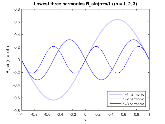
Plot of the individual harmonics
Note the alternating sign
L     = 1;
x     = linspace(-L, L, 80);  % Parition the interval [-L, L] into points
Const = -2*L/pi;              % Constant in the expression for B_n

for n = 1 : 3
    Const = -Const;       % Efficient way to implement alternating sign
    Bn = Const/n;         % Coefficients inversely proportional to n
    Fn = Bn * sin(n*pi*x);
    plot(x, Fn, 'color', [0 0 1] + (3-n)/2.5*[1 1 0], 'linewidth', 3.5-n);
    hold on;
end

xlabel('x'); ylabel('B_nsin(n \pi x/L)');
title('Lowest three harmonics B_nsin(n\pix/L) (n = 1, 2, 3)');
legend('n=1 harmonic', 'n=2 harmonic', 'n=3 harmonic', 'Location', 'Southeast');
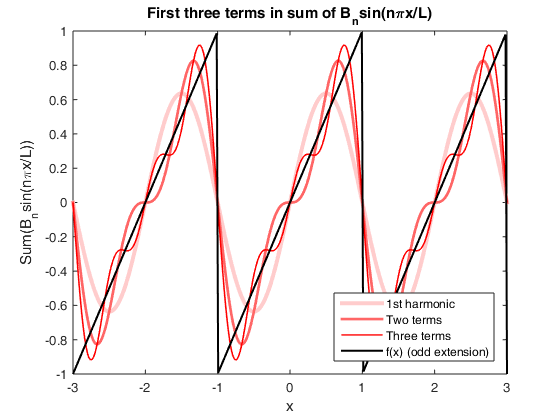
Plot the Fourier series
Now we add the above harmonics: see how they add up to reproduce f(x)=x
hold off;
x     = linspace(-3*L, 3*L, 300); % Enlarge the interval to 3 periods
Const = -2*L/pi;                  % Constant in the expression for B_n
Sn    = zeros(size(x));           % Initialize vector of series sum values

for n = 1 : 3
    Const = -Const;       % Efficient way to implement alternating sign
    Bn = Const/n;         % Coefficients inversely proportional to n
    Fn = Bn * sin(n*pi*x);
    Sn = Sn + Fn;
    plot(x, Sn, 'color', [1 0 0] + (3-n)/2.5*[0 1 1], 'linewidth', 4-n);
    hold on;
end

xlabel('x'); ylabel('Sum(B_nsin(n\pix/L))');
title('First three terms in sum of B_nsin(n\pix/L)');
plot(x, mod(x+1,2)-1,  'k-', 'linewidth', 1.5)
legend('1st harmonic', 'Two terms', 'Three terms', 'f(x) (odd extension)', 'Location', 'Southeast');

% Note how the sum approaches the odd periodic extension of f(x)