Homework 2: Chapter 8, Linear Programming
3.
Objective: Maximize Profit
Decision Variables:
X1 = Number of chairs to be produced next week
X2 = Number of bookshelfs to be produced next week
Objective function: Maximize Z = 15*(X1) + 21*(X2)
Subject to the following constraint functions:
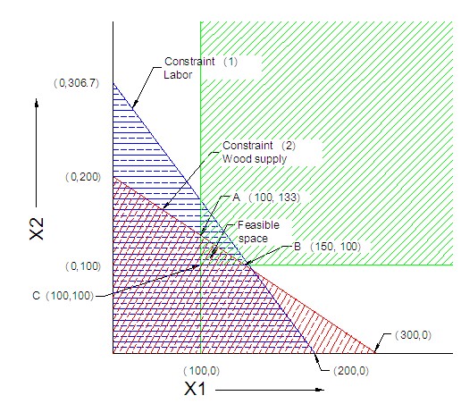
Labor hours availability : 4*(X1) + 3*(X2) ≤ 920 (1)
Wood availability: 8*(X1) + 12*(X2) ≤ 2400 (2)
Policy: X1 ≥ 100 (3)
Policy: X2 ≥ 100 (4)
13.
To plot the constraint functions graphically we first replace the '≤' or '≥' signs by '=' sign. This converts each of the constraint functions from representing an area to line. Then we find the points of intersection of the constraint lines with the X1 and X2 axes.
For example, for the constraint line (1), inserting X1 = 0, we get 4*(0) +
3*(X2) = 920 or X2 = 920/3 = 306.7. This is the intersection point of the line
with the vertical axis X2, with a coordinate (0,306.7).
Similarly, inserting X2=0, we get 4*(X1) + 3*(0) = 920, or X1 = 920/4 = 230.
Thus the other intersecting point on X1 axis is (230,0)
Calculating in a similar manner for the constraint line (2) the two intersecting points are (0,200) and (300,0)
The constrain line (3) and (4) are two lines parallel to X2 and X1 axes, respectively
With these information, the four constraint lines are drawn and then according to '≤' or '≥' signs on the constraint functions, the areas they are representing are indicated by hatched areas.
The feasible space that satisfies all four constrains is the triangle ABC.
Point A is the intersection of line (2) and (3). Thus the point of intersection can be obtained by solving the two equations simultaneously:
8*(X1) + 12*(X2) = 2400 (2)
X1 = 100 (3)
Putting X1=100 in equation (2) we get,
800+12*(X2) = 2400
or, X2 = (2400-800)/12 = 133.3.
Thus the point A has a coordinate (100,133.3)
Point B is the intersection of line (2) and (4):
8*(X1) + 12*(X2) = 2400 (2)
X2 = 100 (4)
Putting X1=100 in equation (2) we get,
800(X1)+12*(100) = 2400
or, X1 = (2400-1200)/8 = 150
Thus the point B has a coordinate (150,100)
The point C is obviously (100,100) and is not expected to be an optimal point. The optimal point will be on the outer periphery of the graph.
Now checking which point maximizes the objective function:
For point A(100, 133.3) : Z = 15*(X1) + 21*(X2) = 15*(100) + 21*(133.3) = 4,300
For point B(150, 100) : Z = 15*(X1) + 21*(X2) = 15*(150) + 21*(100) = 4,350
As Z is maximum at point B, the optimal solution is point B, that is, X1=150, and X2 = 100, and the maximum Z = 4,350.
This means the optimal plan of production next week should be to produce 150 chairs, and 100 bookshelves next week, which should generate a profit of $4,350.
21 (a).
POM software is used to solve the problem.
POM output of LP-A
The optimal solution is to produce 150 chairs (X1) and 100 bookshelves (X2), which will produce a total profit of $4,350.
Slack 1 = 20 means that 20 excess labor hours are available. That is the above optimal solution does not use 20 hours of labor.
Slack 3 = 50 means that the management policy X1 (i.e. # of chairs) ≥ 100 has been exceeded by 50, which we can find from the solution. Thus even if the policy were to produce more than or equal to 150 chairs, there would have been no change in the solution.
Shadow prices:
Shadow price of labor availability is zero, which should be rightly so, because
there is already excess capacity and any additional labor capacity will not
increase the profit.
Shadow price of wood supply = $ 1.875, which is valid for a range of 2000 - 2440. This means that, if everything else remains the same, by increasing wood availability by 1 board feet, the profit will increase by $1.875. And this increase in profit will occur till total wood supply reaches 2440 board feet.
Shadow price for the constraint (3), that is the least number of chairs to be produced is again zero, thus decreasing or increasing this limit up to 150 will not change the solution.
Shadow price for the constraint (4), that is the least number of bookshelves to be produced is $1.5 (within a range of 93.3 to 133.3). This means that if the current minimum limit of production of bookshelves (100) is decreased to 93.3, it would increase the total profit by $1.5 per bookshelf. Similarly if the current minimum limit of production of bookshelves (100) is increased to 133.3, then it would decrease the total profit by $1.5 per bookshelf. These facts are clear from the graphical solution above. Increasing or decreasing the minimum number of bookshelves will cause the horizontal line (X2 = 100) to move up or down, respectively, which in turn will cause the point C to move up and down along the constraint line (2).
4.
Objective: Maximize Profit
Decision Variables:
X1 = Number of hundred gallons of premium ice cream to be produced next week
X2 = Number of hundred gallons of light ice cream to be produced next week
Objective function: Maximize Z = 100*(X1) + 100*(X2)
Subject to the following constraint functions:
Mixing machine availability : 0.3*(X1) + 0.5*(X2) ≤ 140 (1)
Milk availability: 90*(X1) + 70*(X2) ≤ 28,000 (2)
14.
To plot the constraint functions graphically we first replace the '≤' sign by '=' sign. This converts the constraint functions from representing areas to lines. Then we find the points of intersection of the constraint lines with the X1 and X2 axes.
For example, for the constraint line (1), inserting X1 = 0, we get 0.3*(0) +
0.5*(X2) = 140 or X2 = 140/0.5 = 280. This is the intersection point of the line
with the vertical axis X2, with a coordinate (0,280).
Similarly, inserting X2=0, we get 0.3*(X1) + 0.5*(0) = 140, or X1 = 140/0.3 =
466.7.
Thus the other intersecting point on X1 axis is (466.7,0)
Calculating in a similar manner for the constraint line (2) the two
intersecting points are (0,400) and (311.1,0)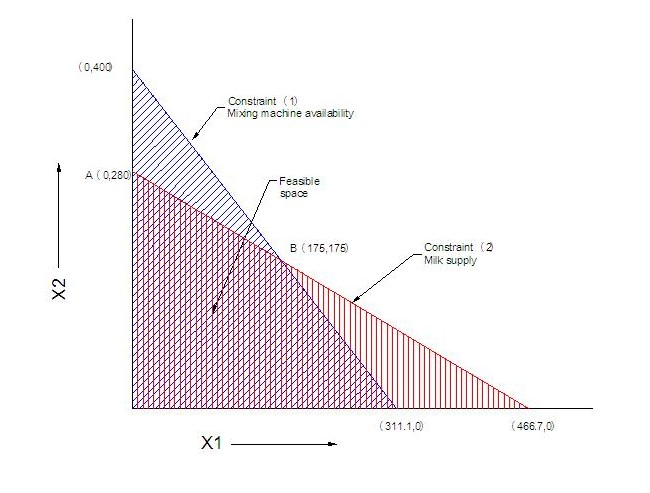
With these information, the two constraint lines are drawn, and then according to '≤' sign on the constraint functions, the areas they are representing are indicated by hatched areas.
The feasible space that satisfies all four constrains is the triangle ABC.
Point A is the intersection of line (1) and X2 axis, which is (0,280)
Point B is the intersection of line (1) and (2). Thus the point of intersection can be obtained by solving the two equations simultaneously:
0.3*(X1) + 0.5*(X2) = 140 (1)
90*(X1) + 70*(X2) = 28,000 (2)
From (1): 0.3*(X1) = 140 -
0.5*(X2)
or ,
X1 = ( 140 - 0.5*(X2))/0.3 (3)
Substituting the value X1 above in equation (2) we get,
90*(( 140 - 0.5*(X2))/0.3) + 70*(X2) = 28,000
or,
42000 - 150*(X2)+70X2 = 28,000
or,
80*(X2) = 42000-28000 = 14,000
or, X2 =
14,000/80 = 175
Substituting X2 in (3):
X1 = ( 140 - 0.5*(175))/0.3 = 175
Thus the point B has a coordinate (175,175)
Point C is the intersection of line (2) with the X1 axis, which is (311.1,0)
Now checking which point maximizes the objective function:
For point A(0, 280) : Z = 100*(X1) + 100*(X2) = 100*(0) + 100*(280) = 28,000
For point B(175, 175) : Z = 100*(X1) + 100*(X2) = 100*(175) + 100*(175) = 35,000
For point C(311.1,0) : Z = 100*(X1) + 100*(X2) = 100*(311.1) + 100*(0) = 31,111
As Z is maximum at point B, the optimal solution is point B, that is, X1=175, and X2 = 175, and the maximum Z = 35,000.
This means the optimal plan of production next week should be to produce 175 hundred gallons of premium ice cream, and 175 hundred gallons of light ice cream, which should generate a profit of $35,000.
21 (b).
POM software is used to solve the problem.
POM output of LP-B
The optimal solution is to produce 175 hundred gallons of premium ice cream, and 175 hundred gallons of light ice cream, which should generate a profit of $35,000.
There is no slack constraint in the solution, which means both the capacities are fully utilized in the solution.
Shadow prices:
Shadow price of constraint 1, (availability of mixing machine) is $83.33, which
is valid for a range of 93.33 to 200 hours. This means that with each hour
increase or decrease of the availability of the mixing machine within the range,
the total profit will increase or decrease by $83.33.
Shadow price of constraint 2, (availability of milk) = $ 0.83, which is valid for a range of 19,600 - 42,000. This means that, if everything else remains the same, by increasing or decreasing milk availability by 1 hundred gallons, the profit will increase or decrease by $0.83, within the given range.
7.
Objective: MINIMIZE TOTAL INGREDIENT COST
Decision Variables:
X1 = Pounds of oats in the hog feed
X2 = Pounds of corns in the hog feed
Objective function: Minimize Z = 0.12*(X1) + 0.07*(X2)
Subject to the following constraint functions:
Mineral needed: 200 X1 + 100 X2 ≥ 3000 (1)
Calorie needed: 200 X1 + 300 X2 ≥ 4000 (2)
Vitamin needed: 100 X1 + 200 X2 ≥ 2000 (3)
17.
For the graphical solution, the intersection points of
three constraints with X2 and X1 axes are as following. (To find how these
points were found see the solution of 13 or 14.)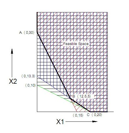
Constraint (1) intersection points with X2 and X1 are:
(0,30) and (15,0)
Constraint (2) intersection points with X2 and X1 are: (0,13.3) and (20,0)
Constraint (3) intersection points with X2 and X1 are: (0,10) and (20,0)
The three constraint areas are drawn and the feasible space is bound by the points A, B and C. Note that the feasible areas are bound by the lines and extends towards right of the line to infinity. Using the coordinates of A, B, and C separately, B minimizes the total cost. The value of Z at B = Z = 0.12*(X1) + 0.07*(X2)
Z= 0.12*12.5+0.07*5 = $ 1.85
That is the optimal solution is to feed the hogs with 12.5 pounds of oats and 5 pounds of corn, which will provide their required nutritional needs in terms of mineral, calorie and vitamin, and it would cost $1.85 per feed, which is minimum.
21 e.
The output essentially gives the same result as discussed above.
The slack in the constraint (3) = 250. Which means that even if the nutritional need in terms of vitamins is increased by 500 units the solution remains unchanged.
The shadow price for constraint 1 is more than the constraint 2. Which indicates that if the mineral requirement is increased, the cost of feed will increase at higher rate.