Lab 4 and Lab 5 Solution
Lab Instructor: Valeria Barra
Contents
- Problem 2: Linear Least Squares Approximation
- Lab 5 Solution
- Lab 5: Problem 1 Polynomial Least Square Approximation of Second Order
- Exercise Sheet Solution
- Exercise 1
- Exercise 2
- Exercise 3
Called Functions
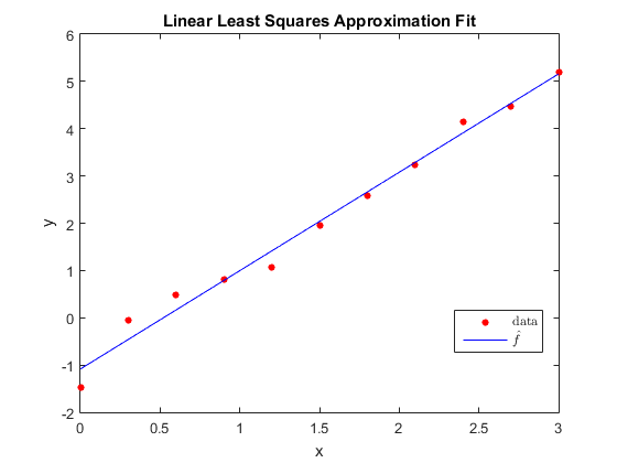
Problem 2: Linear Least Squares Approximation
Do Problem 1 in sec. 7.1 of your textbook. Compare your result with the MATLAB built-in "polyfit" function of the first order. Show your error using formula (7.3) in your textbook. Plot the data points and the fit you found in the same figure.
Solution:
clear all; clc; close all;
% arrays of data points
xi=0:0.3:3;
yi=[-1.466,-0.062,0.492,0.822,1.068,1.944,2.583,3.239,4.148,4.464,5.185];
n=length(yi);

% the sum of the elements xi
sumx1=MySum(xi);
% we need the sum of the xi squars
xi2=xi.^2;
sumx2=MySum(xi2);
% the sum of the yi
sumy1=MySum(yi);
% we need the sum of the xi*yi
xiyi=xi.*yi;
sumx1y1=MySum(xiyi);

% set the linear system in matrix form
A=[n sumx1; sumx1 sumx2];
b=[sumy1; sumx1y1];

% solve the linear system in matrix form using the built-in MATLAB "\" operator:
x=A\b;
fhat=@(t) x(1) + x(2)*t;
SumLeastSquares=MySum(((fhat(xi) - yi)).^2);
Err1= sqrt((1/n)*SumLeastSquares);
fprintf('The Error for the first order approximation is: %10.8e\n',Err1);
%check with Matlab built-in
P=polyfit(xi,yi,1);
fMatlab=polyval(P,xi);
ErrMatlab=norm(fhat(xi)-fMatlab,inf);
fprintf('The Error with Matlab is: %10.8e\n',ErrMatlab);
% an array of x-values to plot the function
xx=0:0.001:3;
plot(xi,yi,'ro','MarkerSize',4,'MarkerFaceColor','r');
hold on
plot(xx, fhat(xx),'b-');
title('Linear Least Squares Approximation Fit')
legend({'data','$\hat{f}$'},'interpreter','latex','Location','best')
xlabel('x')
ylabel('y')
The Error for the first order approximation is: 2.35649032e-01
The Error with Matlab is: 1.77635684e-15
Lab 5 Solution
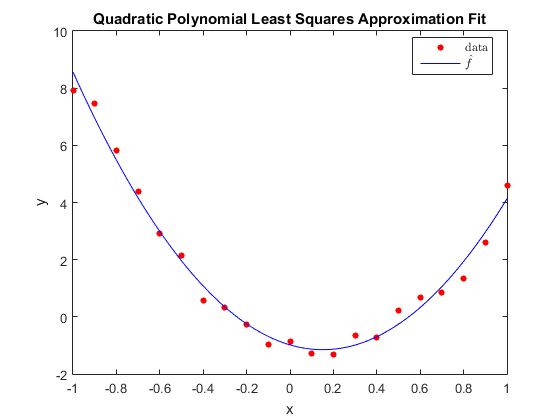
Lab 5: Problem 1 Polynomial Least Square Approximation of Second Order
Do Problem 3 in sec. 7.1 in the textbook.
Solution:
xi=-1:0.1:1;
yi=[7.904, 7.452, 5.827, 4.4, 2.908, 2.144, 0.581, 0.335, - 0.271, -0.963, -0.847, -1.278, -1.335, - 0.656, -0.711, 0.224, 0.689, 0.861, 1.358, 2.613, 4.599];
n=length(yi);

% the sum of the elements xi
sumx1=MySum(xi);
% now we need the sum of the xi squars
xi2=xi.^2;
sumx2=MySum(xi2);
% we need the sum of the xi cubed
xi3=xi.^3;
sumx3=MySum(xi3);
% we need the sum of the xi to the fourth
xi4=xi.^4;
sumx4=MySum(xi4);
% the sum of the yi
sumy1=MySum(yi);
% now we need the sum of the xi*yi
xiyi=xi.*yi;
sumx1y1=MySum(xiyi);
% we need the sum of the xi^2*yi
xi2yi=xi2.*yi;
sumx2y1=MySum(xi2yi);

A=[n sumx1 sumx2;  sumx1 sumx2 sumx3; sumx2 sumx3 sumx4];
b=[sumy1; sumx1y1 ; sumx2y1];
% solve the linear system in matrix form using the built-in MATLAB "\" operator:
x=A\b;

% the canonical basis for quadratic polynomials
phi1=@(t)(1); phi2=@(t)(t); phi3=@(t)(t.^2);
% an array of x-values to plot the function
xx=-1:0.001:1;
Phi1=phi1(xx); Phi2=phi2(xx); Phi3=phi3(xx);
fhat=x(1).*Phi1 + x(2).*Phi2 + x(3).*Phi3;

Phi21=phi1(xi); Phi22=phi2(xi); Phi23=phi3(xi);
fhatErr=x(1).*Phi21 + x(2).*Phi22 + x(3).*Phi23;
SumLeastSquares=MySum(((fhatErr - yi)).^2);
Err2= sqrt((1/n)*SumLeastSquares);
fprintf('The Error for the second order approximation is: %10.8e\n',Err2);
%check with Matlab built-in
P=polyfit(xi,yi,2);
fMatlab=polyval(P,xi);
ErrMatlab=norm(fhatErr-fMatlab,inf);
fprintf('The Error with Matlab is: %10.8e\n',ErrMatlab);
figure;
plot(xi,yi,'ro','MarkerSize',4,'MarkerFaceColor','r');
hold on
plot(xx, fhat,'b-');
title('Quadratic Polynomial Least Squares Approximation Fit')
legend({'data','$\hat{f}$'},'interpreter','latex','Location','best')
xlabel('x')
ylabel('y')
The Error for the second order approximation is: 3.44633215e-01
The Error with Matlab is: 3.55271368e-15
Exercise Sheet Solution
Exercise 1
Problem statement: Write a MATLAB program calculating

Solution:
n=100; % How far we’re summing up to
S=0; % The sum variable S starts out at 0
for k = 0 : n % Loop over values of k from 1 to n
    if mod(k,2) == 0 % if k is even, the next line is executed
        S = S + 1 / factorial(k);
    else % otherwise, k is odd, the following line is executed:
        S = S - 1 / factorial(k);
    end % end of “if” statement
end % end of the for loop
disp( ['for k=', num2str(k), ': the last partial sum equals ', num2str(S) ]);
% Show only the result. the last partial sum
for k=100: the last partial sum equals 0.36788
Note: How do we check that this result is correct? Knowing from Calculus that the series represents the  , in this case with x=1, ie
  .
.
CheckResult=exp(-1);
disp(['the actual sum up to 5 precision digits is: ',num2str(CheckResult)]);
the actual sum up to 5 precision digits is: 0.36788
Exercise 2
Problem statement: Write a MATLAB program calculating  with an error tolerance of 10^(-6).
Solution:
tolerance = 1e-6; % Set the error tolerance to 10^(-4)
S = 0; % The sum variable S starts out at 0
term = 1; % Set to high enough value
k = 0; % first term corresponds to k=0
sgn = 1;
while abs(term) > tolerance % repeat until the next term is less than the
                               % error tolerance
term = sgn / factorial(k); % calculate the next (k-th) term
S = S + term; % add k-th term to the sum variable S
k = k + 1; % increment summation index k (in a “for” loop, this is done
               % automatically)
sgn = -sgn; % this assignment avoids the use of the "if-else" statement
               % used in the previous exercise
end
disp( ['for k=', num2str(k-1), ': the last partial sum equals ', num2str(S) ]);
% Show the final result

% show that we reached the desired tolerance
fprintf(['And we have reched the desired tolerance because the next term '...
'would\n have been:%e. \n'],term); % Note: the three low dots serve to continue
                              % any long matlab command in multiple lines
for k=10: the last partial sum equals 0.36788
And we have reched the desired tolerance because the next term would
 have been:2.755732e-07.
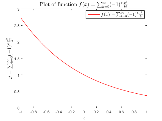
Exercise 3
Problem Statement: Calculate 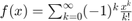 and plot the values of the function for a set of 80 values of x on the interval [-1; 1]
Solution:
N = 80; % Number of points in the plot
X = linspace(-1, 1, N); % Create a set of N values between -1 and 1
Y = zeros(N, 1); % create the corresponding Y array where we store the summation
                       % for each value of little x
tolerance= 1e-5;

for i = 1 : N % Main part of the program: calculate the sum for each of the
                   % N x-values
x = X(i); % Assign the next x-value to the variable x
S = 0; % initialize
k = 0; % first term corresponds to k=0
sgn = 1; % initialize as positive for the first term in the series
term=1; % initialize to a big enough value

    while abs(term) > tolerance % repeat until the next term is less than the
                                   % error tolerance
    % put here all commands needed to calculate the sum “S” for each value of x
    term = (sgn.*(x.^(k))) ./ factorial(k); % calculate the next (k-th) term
        % note: here little x is a scalar, so we don't actually need the .
        % operator, but it is a good practice
    S = S + term; % add k-th term to the sum variable S
    k = k + 1;
    sgn = -sgn; % this assignment avoids the use of the "if-else" statement
                   % used in the previous exercise
    end
Y(i) = S; %; store the result in the appropriate element of the y-array

end
figure; %opens a new figure
plot(X,Y,'r','Linewidth',1)
box on % to put a nice frame around your plot
xlabel('$x$','interpreter','latex','fontsize',14); % label the plot and use
                                              % math fonts in latex
ylabel('$y=\sum_{k=0}^{\infty}(-1)^k \frac{x^k}{k!}$','interpreter','latex',...
    'fontsize',14);
legend({'$f(x)=\sum_{k=0}^{\infty}(-1)^k \frac{x^k}{k!}$'},'interpreter','latex',...
    'fontsize',12,'location','best');
title('Plot of function $f(x) =\sum_{k=0}^{\infty}(-1)^k \frac{x^k}{k!}$',...
    'interpreter','latex','fontsize',14);
Note:
To dsplay the called function "OurFirstFunction.m" using the  Publish option, I have used the "publishdepfun.m" function, that can be downloaded for free from the Mathworks website http://www.mathworks.com/matlabcentral/fileexchange/33476-publish-dependent-and-called-functions
You need to save it in your Current Directory to make sure you can use it. You can use this function to publish your script file together with any auxiliary function you call in that code. Simply type
>> publishdepfun('your_m-file.m',[],{included_functions},{excluded_functions})
in the Command Window.