Lab 6 Solution
Lab Instructor: Valeria Barra
Contents
Due Monday 10/19/15
Problem 1: Euler's Method
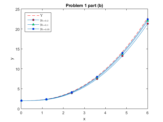
Reproduce tables 8.1 and 8.2 - pg. 382-383 - (about examples 8.2.1 (a) and (b)). Reproduce fig. 8.4 at page 383, but also plot on the same graph the approximations for h=0.1,0.05.
Solution:
clear all; close all;
% a cell array containing the two functions handles for the exercises
f={@(x,y)(-y),@(x,y)((y + x.^2 -2)./(x+1))};
% a cell array containing the two true solutions
Y={@(x)(exp(-x)),@(x)(x.^2 + 2.*x + 2 -2.*(x+1).*log(x+1))};
h=[0.2 0.1 0.05];
% a set of markers and colors for the graphs
Markers = ['o' '^' 's'];
Colors=['r' 'g' 'b' ];
% the ICs given
y0=[1,2];

% strings to be displayed in the headers of the tables
Strings=['a','b'];
Markers = ['o' '^' 's']; % just different symbols to plot
Colors = ['r' 'g' 'b']; % different colors used for the different markers

% the main cycle of the call of the function and display starts here
for k=1:length(f)
    % print the header of the table
    fprintf('\nExecution of Problem 1, part (%s)\n',Strings(k))
    fprintf('_________________________________________________\n\n')
    fprintf('h      x      yh            Error      RelError \n')
    fprintf('_________________________________________________\n')
    for j=1:length(h)
        if k==1
            x{j,:}=(0:h(j):5); % domain for the first part
        else
            x{j,:}=(0:h(j):6); % domain for the second part
        end

        % the call of the method
        y{j,:}=Euler(f{k}, x{j}, y0(k),h(j));
        % plotting only of the second part of the exercise
        if k==2
            if j==1
                plot(x{j,:},Y{k}(x{j,:}),'--r') % plots the real solution only the first time
                hold on
            end
            % plots of all the approximations here
            line_fewer_markers(x{j,:},y{j,:},6,Markers(j),'MarkerFaceColor',Colors(j),'MarkerSize',5);
        end
        % now we only read those values that we want to display
        for i=1/h(j)+1:1/h(j):length(x{j}) % we start by 1/h +1 because of the initial zero, with an increment of 1/h
            Error=Y{k}(x{j}(i)) - y{j}(i);
            RelErr=Error./Y{k}(x{j}(i));
            % print the table
            if i==1/h(j)+1
                fprintf('%3.2f  %2.1g    %6.4e    %4.2e      %5.4f \n', h(j),x{j}(i), y{j}(i) , Error,RelErr)
            else
                fprintf('      %2.1g    %6.4e    %4.2e      %5.4f \n',x{j}(i), y{j}(i) , Error,RelErr)
            end
        end
        fprintf('_________________________________________________\n')
    end
end
% attributes of the figure here
title('Problem 1 part (b)')
xlabel('x')
ylabel('y')
legend({'Y','$y_{h=0.2}$','$y_{h=0.1}$','$y_{h=0.05}$'},'interpreter','latex','location','northwest');
Execution of Problem 1, part (a)
_________________________________________________

h      x      yh            Error      RelError
_________________________________________________
0.20   1    3.2768e-01    4.02e-02      0.1093
       2    1.0737e-01    2.80e-02      0.2066
       3    3.5184e-02    1.46e-02      0.2933
       4    1.1529e-02    6.79e-03      0.3705
       5    3.7779e-03    2.96e-03      0.4393
_________________________________________________
0.10   1    3.4868e-01    1.92e-02      0.0522
       2    1.2158e-01    1.38e-02      0.1017
       3    4.2391e-02    7.40e-03      0.1486
       4    1.4781e-02    3.53e-03      0.1930
       5    5.1538e-03    1.58e-03      0.2351
_________________________________________________
0.05   1    3.5849e-01    9.39e-03      0.0255
       2    1.2851e-01    6.82e-03      0.0504
       3    4.6070e-02    3.72e-03      0.0747
       4    1.6515e-02    1.80e-03      0.0983
       5    5.9205e-03    8.17e-04      0.1213
_________________________________________________

Execution of Problem 1, part (b)
_________________________________________________

h      x      yh            Error      RelError
_________________________________________________
0.20   1    2.1592e+00    6.82e-02      0.0306
       2    3.1697e+00    2.39e-01      0.0700
       3    5.4332e+00    4.76e-01      0.0806
       4    9.1411e+00    7.64e-01      0.0772
       5    1.4406e+01    1.09e+00      0.0705
       6    2.1303e+01    1.45e+00      0.0639
_________________________________________________
0.10   1    2.1912e+00    3.63e-02      0.0163
       2    3.2841e+00    1.24e-01      0.0365
       3    5.6636e+00    2.46e-01      0.0416
       4    9.5125e+00    3.93e-01      0.0397
       5    1.4939e+01    5.60e-01      0.0361
       6    2.2013e+01    7.44e-01      0.0327
_________________________________________________
0.05   1    2.2087e+00    1.87e-02      0.0084
       2    3.3449e+00    6.34e-02      0.0186
       3    5.7845e+00    1.25e-01      0.0212
       4    9.7062e+00    1.99e-01      0.0201
       5    1.5215e+01    2.84e-01      0.0183
       6    2.2381e+01    3.76e-01      0.0165
_________________________________________________
Problem 2: Richardson's Extrapolation
Reproduce table 8.3 at page 392. Compare the error you get according to Richardson's error formula (last column in table 8.3) with the one you got in table 8.1. Comments on the error and on your results.
Solution:
clear all;
f=@(x,y)(-y);
Y=@(x)(exp(-x));
h=0.05;
% the IC given for y
y0=1;
% the first discretization
x1=0:h:5;
% the second discretization with the double step size
x2=0:2*h:5;
% the first call of Euler's method with the first step size
y1=Euler(f, x1, y0,h);
% the second call of Euler's method with the second step size (double)
y2=Euler(f, x2, y0, 2*h);
n=length(x1)-1;
% selected values of x to be displayed
xpos1=x1(1) + n/x1(end) ;
% the header of the table
fprintf('\nExecution of Problem 2\n')
fprintf('___________________________________________________________\n\n')
fprintf(' x    Y-yh       yh-y2h        yRich           ErrorRich \n')
fprintf('___________________________________________________________\n')
for i=1:x1(end)
    xsel(i)=x1(i*xpos1 +1); % another way of selecting only those points that we want to visualize in the table
    % resize y so that we can subtract y2 to it pointwise, but without
    % overwriting the same variable, so that we can read it again at the next loop
    y=y1(i*xpos1 +1);
    Errorh1=Y(x1(i*xpos1 +1)) - y;
    Errorh2=y - y2(i*xpos1/2 +1);
    Richard=2.*y - y2(i*xpos1/2 +1); % now the position to be displayed is halved because y2 has a double spacing 2*h
    ErrRichard=Y(x1(i*xpos1 +1)) - Richard;
    fprintf('%2g  %6.2e    %6.2e    %8.7e      % 8.2e \n',xsel(i), Errorh1,Errorh2,Richard,ErrRichard)
end
fprintf('____________________________________________________________\n')
Execution of Problem 2
___________________________________________________________

 x    Y-yh       yh-y2h        yRich           ErrorRich
___________________________________________________________
 1  9.39e-03    9.81e-03    3.6829340e-01      -4.14e-04
 2  6.82e-03    6.94e-03    1.3544766e-01      -1.12e-04
 3  3.72e-03    3.68e-03    4.9748440e-02       3.86e-05
 4  1.80e-03    1.73e-03    1.8249866e-02       6.58e-05
 5  8.17e-04    7.67e-04    6.6872832e-03       5.07e-05
____________________________________________________________
Comments on results: We can see that this method is more accurate than Euler's scheme. Compare the errror obtained in last column of the last table with the first table (Problem 1 part (a)). It can be proven that this method is of order two, while Euler's explicit scheme is only of order one.