Lab 11 Solution
Lab Instructor: Valeria Barra
Contents
DUE Tuesday 04-19-2016 ;
Problem 1: Runge-Kutta 4
Implement your own RK-2 and RK-4 methods to solve the same IVP seen last week. Reproduce the table, showing the grid points  , approximated solution
  , the actual solution
  and the error
  , all at the same grid points
  . To compute the error at each grid point
  use the value for the actual solution given
 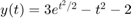 .
.
Solution:
clear all; close all;
% function handle of the RHS function for the problem
f=@(t,y)(t.*y + t.^3);
% the actual solution
y=@(t)( 3*exp((t.^2)./2) - t.^2 -2);
h=[0.2 0.1 0.05];

% the IC given
w0=1;

Colors = ['c' 'g' 'b']; % different colors used for the different curves
Styles = [':', '--', '.-']; % different line styles used for the different curves

% the main cycle of the call of the function and display starts here
for j=1:length(h)
    t{j}=(0:h(j):1); % domain
    % the call of the methods
    wRK2{j}=RungeKutta2(f, t{j}, w0,h(j));
    wRK4{j}=RungeKutta4(f, t{j}, w0,h(j));
    % plots of all the approximations here
    figure(1) % opens a new figure and labels it as figure 1
    hold on
    plot(t{j},wRK2{j},'linestyle',Styles(j),'color',Colors(j),'linewidth',2);

    figure(2) % opens a new figure and labels it as figure 2
    plot(t{j},wRK4{j},'linestyle',Styles(j),'color',Colors(j),'linewidth',2);
    hold on
end


% plot of actual solution here
figure(1)
plot(t{j},y(t{j}),'--r','linewidth',2) % plots the real solution only once
% attributes of the figure 1 here
title('Problem 1: RK-2')
xlabel('t')
ylabel('w')
box on
legend({'$w_{h=0.2}$','$w_{h=0.1}$','$w_{h=0.05}$','y'},'interpreter','latex','fontsize',16,'location','northwest');
figure(2)
plot(t{j},y(t{j}),'--r','linewidth',2) % plots the real solution only once
% attributes of the figure 2 here
title('Problem 1: RK-4')
xlabel('t')
ylabel('w')
box on
legend({'$w_{h=0.2}$','$w_{h=0.1}$','$w_{h=0.05}$','y'},'interpreter','latex','fontsize',16,'location','northwest');

% now we only read those values that we want to display
for i=1:length(h)
        TPrint{i}=t{i}(1:h(1)/h(i):end); % select only the values we want to print in the table
        WRK2Print{i}=wRK2{i}(1:h(1)/h(i):end); % select only the values we want to print in the table
        WRK4Print{i}=wRK4{i}(1:h(1)/h(i):end); % select only the values we want to print in the table
    if i==length(h)
        ErrorRK2=abs(y(TPrint{i}) - WRK2Print{i}); % error calculated point-wise only with the third execution
        ErrorRK4=abs(y(TPrint{i}) - WRK4Print{i}); % error calculated point-wise only with the third execution
    end

end

% table for RK-2
fprintf('\nExecution of Problem 1, RK-2 \n')
fprintf('__________________________________________________________________________________________\n\n')
fprintf('t        w_{h=0.2}(t_i)  w_{h=0.1}(t_i)  w_{h=0.05}(t_i)     y_i       Error w_{h=0.05} \n')
fprintf('__________________________________________________________________________________________\n')

% print the table
tableRK2=[(TPrint{1,3})' (WRK2Print{1,1})' (WRK2Print{1,2})' (WRK2Print{1,3})' (y(TPrint{1,3}))' (ErrorRK2)'];
fprintf('%2.1f        %6.4f          %6.4f          %6.4f          %6.4f          %6.4e \n',tableRK2')
%end of table line
fprintf('__________________________________________________________________________________________\n')

% table for RK-4
fprintf('\nExecution of Problem 1, RK-4 \n')
fprintf('__________________________________________________________________________________________\n\n')
fprintf('t        w_{h=0.2}(t_i)  w_{h=0.1}(t_i)  w_{h=0.05}(t_i)     y_i       Error w_{h=0.05} \n')
fprintf('__________________________________________________________________________________________\n')

tableRK4=[(TPrint{1,3})' (WRK4Print{1,1})' (WRK4Print{1,2})' (WRK4Print{1,3})' (y(TPrint{1,3}))' (ErrorRK4)'];
fprintf('%2.1f        %6.4f          %6.4f          %6.4f          %6.4f          %6.4e \n',tableRK4')
%end of table line
fprintf('__________________________________________________________________________________________\n')


pRK2= log2((WRK2Print{1,2}(end) - WRK2Print{1,1}(end))/(WRK2Print{1,3}(end) - WRK2Print{1,2}(end)));
fprintf('The order of converegnce of RK-2 at the point t_i = 1 is p = %4.2f. That is roughly 2.\n',pRK2)

pRK4= log2((WRK4Print{1,2}(end) - WRK4Print{1,1}(end))/(WRK4Print{1,3}(end) - WRK4Print{1,2}(end)));
fprintf('The order of converegnce of RK-4 at the point t_i = 1 is p = %4.2f. That is roughly 4.\n',pRK4)
Execution of Problem 1, RK-2
__________________________________________________________________________________________

t        w_{h=0.2}(t_i)  w_{h=0.1}(t_i)  w_{h=0.05}(t_i)     y_i       Error w_{h=0.05}
__________________________________________________________________________________________
0.0        1.0000          1.0000          1.0000          1.0000          0.0000e+00
0.2        1.0208          1.0207          1.0206          1.0206          2.1478e-05
0.4        1.0909          1.0902          1.0899          1.0899          8.7939e-05
0.6        1.2340          1.2323          1.2318          1.2317          1.8449e-04
0.8        1.4949          1.4924          1.4917          1.4914          2.7374e-04
1.0        1.9494          1.9471          1.9464          1.9462          2.6690e-04
__________________________________________________________________________________________

Execution of Problem 1, RK-4
__________________________________________________________________________________________

t        w_{h=0.2}(t_i)  w_{h=0.1}(t_i)  w_{h=0.05}(t_i)     y_i       Error w_{h=0.05}
__________________________________________________________________________________________
0.0        1.0000          1.0000          1.0000          1.0000          0.0000e+00
0.2        1.0206          1.0206          1.0206          1.0206          2.5901e-09
0.4        1.0899          1.0899          1.0899          1.0899          1.0193e-08
0.6        1.2316          1.2317          1.2317          1.2317          2.2996e-08
0.8        1.4914          1.4914          1.4914          1.4914          4.4549e-08
1.0        1.9461          1.9462          1.9462          1.9462          9.0354e-08
__________________________________________________________________________________________
The order of converegnce of RK-2 at the point t_i = 1 is p = 1.67. That is roughly 2.
The order of converegnce of RK-4 at the point t_i = 1 is p = 4.02. That is roughly 4.
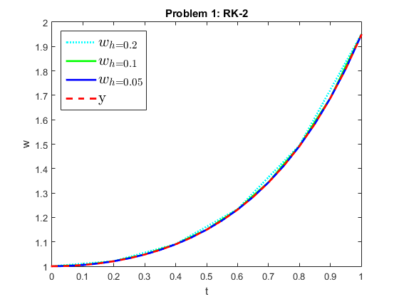

Comments on results: From the values for each row in the two tables, we can see that RK-2 scheme is of order two locally. In fact, as h is halved for each execution, the corresponding error for each grid point is roughly divided by four. Whereas RK-4 scheme is of order four locally. In fact, as h is halved for each execution, the corresponding error for each grid point is roughly divided by sixteen. Whereas Euler forward method was only of order one. This can also be seen from the p value. The figures look almost identical, except for the one for RK-4 that starts, even with the the coarsest approximation, closer to the actual solution.