Lab 6 Solution

Lab Instructor: Valeria Barra DUE Tuesday 03-01-2016

Contents

First Problem: Interoplation with Chebyshev Nodes

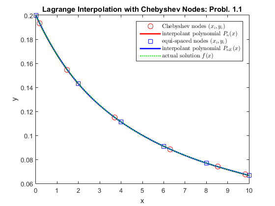
Problem 1.1)

Consider the interpolating polynomial for f(x)= 1 / (x+5) with interpolation Chebyshev nodes on [0,10]. Find an upper bound for the interpolation error at x=1 and x=5.

clear all;
close all;
disp('Execution of Probl. 1.1)')
% the set of data points given in the problem is not equi-spaced, but we
% need to find the Chebyshev nodes
n = 6; % the number of data points
a = 0; b = 10;
xi = ChebyNodes(n,a,b); % call to the function that calculates the Chebyshev nodes

% now to compare the performance with the equi-spaced points
xiE= a:2:b;
f = @(x)(1 ./ (x+5)); % the function given
yi=f(xi); % evaluate the f-values of the Chebyshev nodes
yiE=f(xiE); % evaluate the f-values of the equi-spaced nodes
% the domain needed for plotting
x=linspace(a,b,101);
% stepsize of the domain is calculated to figure out which points to select for the error
domstepsize=(x(end)-x(1))/(length(x)-1);
% call to the function with Chebyshev nodes
p= LagrangeInterpolation(xi,yi,x);
% call to the function with equi-spaced nodes
pE= LagrangeInterpolation(xiE,yiE,x);

figure; % starts a new figure
plot(xi,yi,'or','MarkerSize',8);
hold on
plot(x,p,'-r','Linewidth',2)
plot(xiE,yiE,'sb','MarkerSize',8);
hold on
plot(x,pE,'-b','Linewidth',2)
hold on
plot(x,f(x),':g','Linewidth',1.5)
title('Lagrange Interpolation with Chebyshev Nodes: Probl. 1.1')
xlabel('x')
ylabel('y')
legend({'Chebyshev nodes $(x_i,y_i)$','interpolant polynomial $P_n(x)$','equi-spaced nodes $(x_i,y_i)$','interpolant polynomial $P_{nE}(x)$','actual solution $f(x)$'},'interpreter','latex')

indexfor1 = ((1 - x(1))/domstepsize) +1;
indexfor5 = ((5 - x(1))/domstepsize) +1;
Err_x1 = abs(p(indexfor1) - f(x(indexfor1))); % the error at x = 1
Err_x5 = abs(p(indexfor5) - f(x(indexfor5))); % the error at x = 5
disp(['The error at x = 1 is ',num2str(Err_x1)])
disp(['The error at x = 5 is ',num2str(Err_x5)])


% now we calculate the max of the theoretical error
Fsym = sym(f);
DerF = diff(Fsym,n);
MaxDerF = max(abs(double(subs(DerF,x))));

% formula for the error bound
ErrorBound = ( (( ((b-a)/2)^n)*MaxDerF ) / ((2^(n-1))* factorial(n)) );
disp(['The estimate of the theoretical error is ',num2str(ErrorBound)])


if ((Err_x1 <= ErrorBound) && (Err_x5 <= ErrorBound))
   disp('We are below the theoretical error. Yay!')
end

Execution of Probl. 1.1)
The error at x = 1 is 9.2794e-05
The error at x = 5 is 7.4019e-05
The estimate of the theoretical error is 0.00625
We are below the theoretical error. Yay!

Problem 1.2)

Consider using 5 Chebyshev nodes points on [0,2] to approximate

disp('Execution of Probl. 1.3)')
a = 0; b = 2;
n = 5; % the number of data points
xi = ChebyNodes(n,a,b); % call to the function that calculates the Chebyshev nodes

% the equispaced nodes to compare the performances
xiE = linspace(0,2,5);
f = @(x)(exp(-3.*x));
yi=f(xi); % evaluate the f-values of the Chebyshev nodes
yiE=f(xiE); % evaluate the f-values of the equi-spaced nodes
x = linspace(a,b,101); % domain
domstepsize=(x(end)-x(1))/(length(x)-1); % stepsize for the domain
% call to the function with Chebyshev nodes
p = LagrangeInterpolation(xi,yi,x);
% call to the function with equi-spaced nodes
pE= LagrangeInterpolation(xiE,yiE,x);

figure; % starts a new figure
plot(xi,yi,'or','MarkerSize',8);
hold on
plot(x,p,'-r','Linewidth',2)
plot(xiE,yiE,'sb','MarkerSize',8);
hold on
plot(x,pE,'-b','Linewidth',2)
hold on
plot(x,f(x),':g','Linewidth',1.5)
title('Lagrange Interpolation with Chebyshev Nodes: Probl. 1.3')
xlabel('x')
ylabel('y')
legend({'Chebyshev nodes $(x_i,y_i)$','interpolant polynomial $P_n(x)$','equi-spaced nodes $(x_i,y_i)$','interpolant polynomial $P_{nE}(x)$','actual solution $f(x)$'},'interpreter','latex')

indexfor02 = ((0.2 - x(1))/domstepsize )+ 1;
P02= p(indexfor02);
f02= f(x(indexfor02));
Err = abs(P02 - f02);
disp(['The error at x=0.2 is = ',num2str(Err)])


% now we calculate the max of the theoretical error
Fsym = sym(f);
DerF = diff(Fsym,n);
MaxDerF = max(abs(double(subs(DerF,x))));

% formula for the error bound
ErrorBound = ( (( ((b-a)/2)^n)*MaxDerF ) / ((2^(n-1))* factorial(n)) );
disp(['The estimate of the theoretical error is ',num2str(ErrorBound)])


if ((Err <= ErrorBound))
   disp('We are below the theoretical error. Yay!')
end

Execution of Probl. 1.3)
The error at x=0.2 is = 0.012666
The estimate of the theoretical error is 0.12656
We are below the theoretical error. Yay!

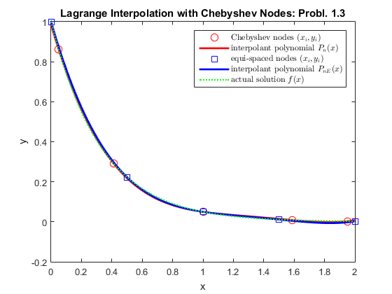
Conclusions: Comparing to the executions from Lab 5, we see that interpolation using Chebyshev nodes has overall a better error (not at x=5 for Probl. 1.1).

Published with MATLAB® R2015a

function xi = ChebyNodes( n,a,b )
% Input arguments:
% - n, the number of Chebyshev nodes we want to find (to calculate an (n-1)-degree interpolating polynomial)
% - a, b, the endpoints of the interval [a,b]
% Ouput argument:
% - xi, the Chebyshev nodes found

% to find the Chebyshev nodes
for i = 1: n
    xi(i)=((a+b)/2) + ((b-a)/2)*cos( ((2*i -1)*pi)/(2*n) );
end
% flip the array xi, since with this construction they are in decresent
% order
xi = fliplr(xi);

end

Published with MATLAB® R2015a

function [p] = LagrangeInterpolation(xi,yi,x)
% data given:
% - x is the vector for the domain on which we will plot the polynomial
% - xi set of first coordinates of data points
% - yi set of second coordinates of data points

p = zeros(1,length(x)); %initialize the vector for the polynomial
for i = 1:length(xi)
    Li = 1; % initialize the L variable for the Lagrange interpolant
    for j = 1:length(xi)
        if i ~= j
            Li = Li.*((x-xi(j))./(xi(i)-xi(j)));
        end
    end
    p = p + Li.*yi(i);
end

end

Published with MATLAB® R2015a