Lab 7 Solution

Lab Instructor: Valeria Barra DUE Tuesday 03-08-2016

Called Functions

ChebyNodes
LagrangeInterpolation

First Problem: Interoplation with Clamped Splines

Problem 1)

Consider the interpolating clamped spline polynomial for $f(x)= \frac{1}{ (1+25 x^2)}$ with 11-equispaced points on [-1,1].

clear all;
close all;
disp('Execution of Probl. 1)')
% the set of data points given in the problem is not equi-spaced, but we
% first define the interval and the nodes
n = 11; % the number of data points
a = -1; b = 1;
xi = linspace(a,b,n);
% define the function symbolically
syms x;
f = 1./(1 + 25.*(x.^2));
Df = diff(f);
% find the derivative at the endpoints
vl = double(subs(Df,{x},a));
vr = double(subs(Df,{x},b));
% now find the y-values
yi = double(subs(f,{x},xi));
% now use the command spline to find the coeddicients of interpolation
cs = spline(xi, [vl yi vr]);
% define a domain
domain = linspace(a,b,101);
% now find the f-values of the interpolating polynomial
pS = ppval(cs,domain);


% now repeat the exercise with Chebychev nodes
xiC = ChebyNodes(n,a,b); % call to the function that calculates the Chebyshev nodes
yiC = double(subs(f,{x},xiC));
% call to the function with Chebyshev nodes
pC= LagrangeInterpolation(xiC,yiC,domain);
% now to compare the performance with the equi-spaced points Lagrangian
% interpolation

% call to the function with equi-spaced nodes
pL= LagrangeInterpolation(xi,yi,domain);

figure; % starts a new figure
plot(xi,yi,'or','MarkerSize',8);
hold on
plot(domain,pS,'-r','Linewidth',2)
hold on
plot(domain,pC,'--b','Linewidth',2)
hold on
plot(domain,pL,':g','Linewidth',2)
hold on
F = double(subs(f,{x},domain));
plot(domain,F,'.-k','Linewidth',1.5)
title('Interpolation with Clamped Splines')
xlabel('x')
ylabel('y')
legend({'nodes $(x_i,y_i)$','$P_S(x)$','$P_C(x)$','$P_L(x)$','actual solution $f(x)$'},'interpreter','latex')

Err_S = max(abs(pS -F)); % the error with P_S
Err_C = max(abs(pC -F)); % the error with P_C
Err_L = max(abs(pL -F)); % the error with P_L
disp(['The max error with the cubic spline is ',num2str(Err_S)])
disp(['The max error with the Chebyshev nodes polynomial is ',num2str(Err_C)])
disp(['The max error with the Lagrange polynomial is ',num2str(Err_L)])

Execution of Probl. 1)
The max error with the cubic spline is 0.021955
The max error with the Chebyshev nodes polynomial is 0.10893
The max error with the Lagrange polynomial is 1.9156

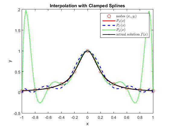
Conclusions: Comparing to the executions, we see that interpolation using the cubic spline is better than the one using Chebyshev nodes and Lagrange, respectively. Lagrange's polynomial highly oscillates towards the boundary of the domain, due to the fact that the nodes are not wisely distributed and it is a 10^th degree polynomial. Chebyshev does a better job fixing these oscillations, but still it is a 10^th degree polynomial. This behavior is totatlly controlled by the spline polynomial instead, since the max degree in each subinterval is 3.

function xi = ChebyNodes( n,a,b )
% Input arguments:
% - n, the number of Chebyshev nodes we want to find (to calculate an (n-1)-degree interpolating polynomial)
% - a, b, the endpoints of the interval [a,b]
% Ouput argument:
% - xi, the Chebyshev nodes found

% to find the Chebyshev nodes
for i = 1: n
    xi(i)=((a+b)/2) + ((b-a)/2)*cos( ((2*i -1)*pi)/(2*n) );
end
% flip the array xi, since with this construction they are in decresent
% order
xi = fliplr(xi);

end

function [p] = LagrangeInterpolation(xi,yi,x)
% data given:
% - x is the vector for the domain on which we will plot the polynomial
% - xi set of first coordinates of data points
% - yi set of second coordinates of data points

p = zeros(1,length(x)); %initialize the vector for the polynomial
for i = 1:length(xi)
    Li = 1; % initialize the L variable for the Lagrange interpolant
    for j = 1:length(xi)
        if i ~= j
            Li = Li.*((x-xi(j))./(xi(i)-xi(j)));
        end
    end
    p = p + Li.*yi(i);
end

end

Lab 7 Solution

Contents

Called Functions

First Problem: Interoplation with Clamped Splines

Problem 1)