|
Final Exam - Matlab Part |
| 1 |
stephensen.m |
Matlab function stephensen(f, x0, tol) calculates the root of equation
f(x)=0, using initial condition x0.
execute stephensen( inline('exp(-x)-x'), 1, 1e-8 );
|
| 2 |
dice.m |
Matlab function dice(diceSum, nTrials) calculates the average number of two-dice rolls
required to get a sum of diceSum, using a Monte-Carlo simulation with nTrials
trials. Execute dice(4, 100), dice(4, 1000) and dice(4, 1000).
Exact result is 12.
|
| 3a,b |
rule3_8.m |
Function rule3_8(f, a, b, N) calculates the integral of inline function
f from a to b using the 3/8 rule with N subintervals.
|
|
problem3.m |
Matlab code for problem 3. The exact slope of the line is -1.5, indicating that the error decreases
as N-3/2.
Note that the convergence to exact solution would be much faster if the integrand did not have an infinite derivative at
x=0. In general, the error of the 3/8 rule decreases as N-5 (faster than for the Simpson's rule)
|
| Homework #4 |
| 1a |
hw4_1.m |
Table comparing f(x)=.5 x2 ((x-1)-1-(x+1)-1) and
g(x)=x2 (x2 - 1)-1 |
| 1b |
g(x) is clearly more accurate - it gives a correct limit of 1 as x -> Inf,
and remains greater than 1 (see table).
f(x) gives poor
results since it contains a difference of two decreasing values. Even a small round-off error
becomes significant as this difference gets smaller and smaller.
|
| 2a |
binomial.m |
Matlab function calculating explicitly the binomial expansion (x + y)n |
| 2b |
hw4_2b.m |
Table of (x+y)15 values calculated using binomial.m, for x=1:20, and y=1-x
|
| For n=15, the binomial expansion only works when x < 7, since it
involves powers of x and y up to 15, which are very large for x ≥ 7.
For instance when x=7, the k=7 term is larger than 1015
( |a7| = x8 y7 15! / (7! 8!) = 1.04 * 1016 ),
resulting in a loss of significance of order one, so the error is comparable to the total sum.
|
| 2c |
hw4_2c.m |
Table of (x+y)n values calculated using binomial.m, for n=1:20, x=10, and y=-9
|
| For x=10 and y=-9, the binomial expansion only works when n < 14, as we
would expect, since loss of significance becomes comparable to one when terms become larger than
1015. When n=14, the k=7 term is |a7| = 107 97 14! / (7! 7!) = 1.64 * 1017
|
| 3 |
mySin.m |
Matlab function calculating sin(x) by summing the Taylor series |
| hw4_3.m |
Table comparing mySin(x) to built-in sin(x) values, for x=0:0.1:pi. Note the almost perfect agreement between the two columns |
| hw4_3b.m |
Comparison for larger angles: mySin(x) fails for x around 35-40 radian. This is because the terms in the Taylor series
are becoming very large as x increases (larger than 1015),
leading to round-off errors comparable in value to the sum itself |
| Homework #5 |
| 1a |
hw5_1a.m |
Table of trigonometric error sin(1+πn)+sin(1), where n is an odd integer.
|
| 1b |
Equation sin(x + πn)+sin(x)=0 will fail miserably when all information about x in
sin(x + πn) is lost. This happens when the round-off error in representing πn becomes comparable to
x. The round-off error of πn is less than 10-15πn.
Therefore, the problem occurs when x < 10-15πn, which for x=1 is satisfied
when n > 1e15 (we don't have to be too accurate here, since we only know the upper bound on error, and not its exact
magnitude).
Let's check using Matlab:
calculation sin(1+pi*(1e15+1))+sin(1) yields -0.06, which may seem tolerable,
but for a slightly higher n=2e15+1
we get sin(1+pi*(2e15+1))+sin(1)=0.47, which definitely represents complete failure.
|
| 1c |
newSin.m |
Matlab function calculating the sine using its Taylor series. The argument is normalized to lie in the interval (-π, π)
before the series is summed, improving the results for large values of the angle.
|
| hw5_1c.m |
Table of trigonometric error sin(1+πn)+sin(1),
where n=10m+1, and m=1:17, for the built-in sine and the newSin functions. This program
also plots the logarithm of this error vs. m (which itself is the log10 of n). The complete failure occurs when log(error)
is close to zero, since this corresponds to error of order one. On the graph this clearly corresponds to m of about 15-16.
|
| 2a |
hw5_2a.doc |
Proof of limit (1+x/N+(x/N)2/2)N -> exp(x) as x -> Infinity
|
| 2b |
limExp.m |
Matlab function calculating the exponential function using the limit calculation. Note the funny header:
this function will return two numbers - the value of the exponential function, and the highest value of m
used to find it.
|
| 2c |
hw5_2c.m |
Comparison of limExp(x) to the built-in function exp(x), for x from 1 to 20. Note the interestingly sudden failure at x=18.
|
The explanation for failure at x=18 is simple: as x increases, higher and higher N is needed to calculate the
limit (see how m grows with increasing x). In fact, we know when the expression under the limit will
fail completely: this will happen when x/N will be of order 1e-15 to 1e-16, since we know
that such a small number will get completely rounded off when added to 1. Now, for x between 10 and
20, this occurs when N > 1e16 or 1e17, which corresponds to 2^53 to 2^56.
From the table you can see that this is exactly the region of m values where the method failed!
|
| Homework #9 |
| 1, 3 |
plotRicker.m |
Matlab function plotRicker(r, y0, n, s) directly computes and plots the solution of the Ricker's equation
with parameter r, initial condition y0=y0, for n steps, using line type s.
|
| 1 |
hw9_1.m |
Plots the directly computed solution to the Ricker's equation for r=2.2, r=2.4, and r=3.4.
|
| 2 |
hw9_2.m |
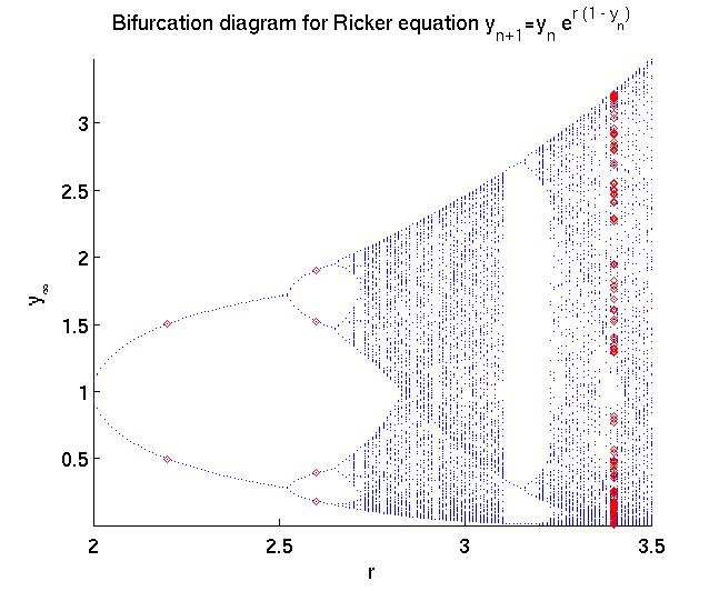
This Matlab function calculates the bifurcation diagram for the Ricker equation yn+1=yn er (1 - yn)
|
| hw9_2.jpg |
The bifurcation diagram for the Ricker equation; note the similarity with the
logistic equation bifurcation diagram
|
| 3 |
hw9_3.m |
The "butterfly effect": note how the slight difference in initial condition is amplified as n grows.
|
| 4 |
butterfly.m |
Matlab function butterfly(y0, d, r) returns the iteration number at which the solutions of the Ricker's equation with parameter r
and initial conditions y0 and y0+d deviate by 0.1 or more.
|
| hw9_4.m |
Predictive power (number of iterations before deviations accumulate) vs. accuracy in specifying initial conditions for the Ricker equation
in chaotic regime (r=4).
|
| 5 |
With double precision accuracy, we cannot trust the computation yn+1=yn e4 (1 - yn)
for more than 74 steps. The curve nd vs. m is approximately linear, with a slope between 4.5 and 4.9 (see plot produced by hw9_4.m).
Therefore, in order to predict (calculate) the value of y500, we need between 500/5 = 100 and
500/4.7 = 106 significant digits.
|
| Homework #10 |
| 1a |
Newton.m |
Matlab function Newton(f, df, x0, tol) calculates the root of any equation
f(x)=0 with the derivative given by funtion df(x) = f '(x).
To find the root of equation cos(x) = x2, using initial condition
x0=1 and tolerance of 10-9, execute the command
Newton( inline('x^2-cos(x)'), inline('2*x+sin(x)'), 1, 1e-9 );
|
| NewtonSym.m |
Optional: same as above, but this program uses Matlab's symbolic capabilities (the Maple core) to calculate the derivative.
Execute the commands
x = sym('x'); Newton(x^2-cos(x), 1, 1e-9 );
|
| 1b |
Bisection.m |
Matlab function Bisection(f, a, b, tol) calculates the root of equation
f(x)=0 bracketed by the interval [a,b].
To find the root of equation cos(x) = x2 between a=0 and b=π/2,
with a tolerance of 10-9, execute the command
Bisection( inline('x^2-cos(x)'), 0, pi/2, 1e-9 );
|
| 1c |
FalsePos.m |
Matlab function FalsePos(f, a, b, tol) calculates the root of equation
f(x)=0 bracketed by the interval [a,b], using the method of false position.
Execute the command
FalsePos( inline('x^2-cos(x)'), 0, pi/2, 1e-9 );
|
| 1d |
Let's now choose the g(x) function for the iteration method: g(x) = x + C f(x) = x + C(x2 - cos x),
so g'(x) = 1 + C(2 x + sin x). Stability condition is -1<g'(xroot)<1 .
In fact, we know that the convergence of a difference
equation is the fastest when g'(xroot) is close to zero: 1 + C(2 xroot + sin xroot) = 0,
which yields C = -1 / (2 xroot + sin xroot) . Now, we know that 0<xroot<π/2
and 0<sin xroot<1. To get a rough estimate for C, let's take the values in the
middle of these intervals: xroot ~ π/4, sin xroot ~ 1/2, so 2 xroot + sin xroot ~ π/2 + 1/2 ~ 2,
yielding C = -1/2 (this is a crude approximation, but it's sufficient)
|
| Iteration.m |
Matlab function Iteration(f, x0, tol) calculates the root of equation
f(x)=0 using the method of iterations. Execute the command Iteration(inline('x-(x^2-cos(x))/2'), 1, 1e-9);
|
| 3 |
ConvOrder.m |
Matlab function ConvOrder(error) makes the plot of ln(εn+1) vs. ln(εn),
using an array of error values ("error"), and calculates the order of convergence of a given method, using
the first and last point on the plot. You must save this function into your Matlab directory before running the programs below
|
| 2a, 3 |
NewtonE.m |
Matlab function NewtonE(f, df, x0, tol, exact) is similar to Newton(f, df, x0, tol) (see above), but uses
the exact root ("exact") to find the convergence order of the method.
To find the order of convergence of the Newton method for equation x2-7=0, using initial condition
x0=1 and tolerance of 10-9, execute the command
NewtonE( inline('x^2-7'), inline('2*x'), 1, 1e-9, sqrt(7) );
|
| 2b, 3 |
BisectionE.m |
Function BisectionE(f, a, b, tol, exact) is similar to function Bisection(f, a, b, tol) (see above),
but uses the exact root to find the convergence order of the bisection method.
Execute the command
BisectionE( inline('x^2-7'), 2, 3, 1e-9, sqrt(7) );
|
| 2c, 3 |
FalsePosE.m |
Same as above, but for a false position method. Execute the command
FalsePosE( inline('x^2-7'), 2, 3, 1e-9, sqrt(7) );
|
| 2d, 3 |
Let's choose the g(x) function for the iteration method: g(x) = x + C f(x) = x + C(x2-7),
so g'(x) = 1 + 2 C x. Stability condition -1 < g'(xroot) < 1 becomes
-1 < 1 + 2 C xroot < 1 . Therefore, -2 < 2 C xroot < 0 , which yields
-1 < C xroot < 0 . Thus, C is a negative constant satisfying C > -1/xroot = -1/sqrt(7) = -0.378.
The following simple choices will work: C=-1/4, -1/5, -1/6, -1/7... The best choice is the one yielding g'(xroot)=0:
C = -1 / (2 xroot) ~ -0.189 ~ -1/5
|
| IterationE.m |
Function IterationE(f, x0, tol, exact) calculates the root of equation
f(x)=0 and finds the order of convergence of the iteration method.
Execute the command IterationE(inline('x-(x^2-7)/5'), 3, 1e-9, sqrt(7));
|
| Homework #11 |
| 1-3 |
midpoint.m |
Function midpoint(a, b, f, N) calculates the integral of inline function
f from a to b using the midpoint rule with N subintervals.
Call example: midpoint(0, pi/2, inline('cos(x.^2)'), 10);
|
|
trapezoid.m |
Function trapezoid(a, b, f, N) calculates the integral of inline function
f from a to b using the trapezoid rule with N subintervals.
Call example: trapezoid(0, pi/2, inline('cos(x.^2)'), 10);
|
|
simpsons.m |
Function simpsons(a, b, f, N) calculates the integral of inline function
f from a to b using the simpsons rule with N subintervals.
Call example: simpsons(0, pi/2, inline('cos(x.^2)'), 10);
|
| 1 |
hw11_1.m |
Comparison of the three intergration methods in calculating the integral of cos(x2)
from 0 to π/2.
|
| 2-3 |
hw11_2.m |
Comparison of the three intergration methods in calculating the integral of ln x
from 1 to 3. Produces a plot and determines the convergence of the
error.
|
|
Jan 19 |
fprintf statement: some examples |
|
Jan 24 |
Making plots: an example |
|
Feb 7 |
Integrating exp(-x2) using the Taylor series |
|
Feb 9 |
Recursive and non-recursive exponential functions |
|
Feb 16 |
Round-off errors, binary system, infinities, and NaN's |
|
Feb 28 |
Solving difference equations: Fibonacci numbers |
|
Mar 2 |
Review of round-off errors and loss of significance (Word doc file) |
|
Mar 28 |
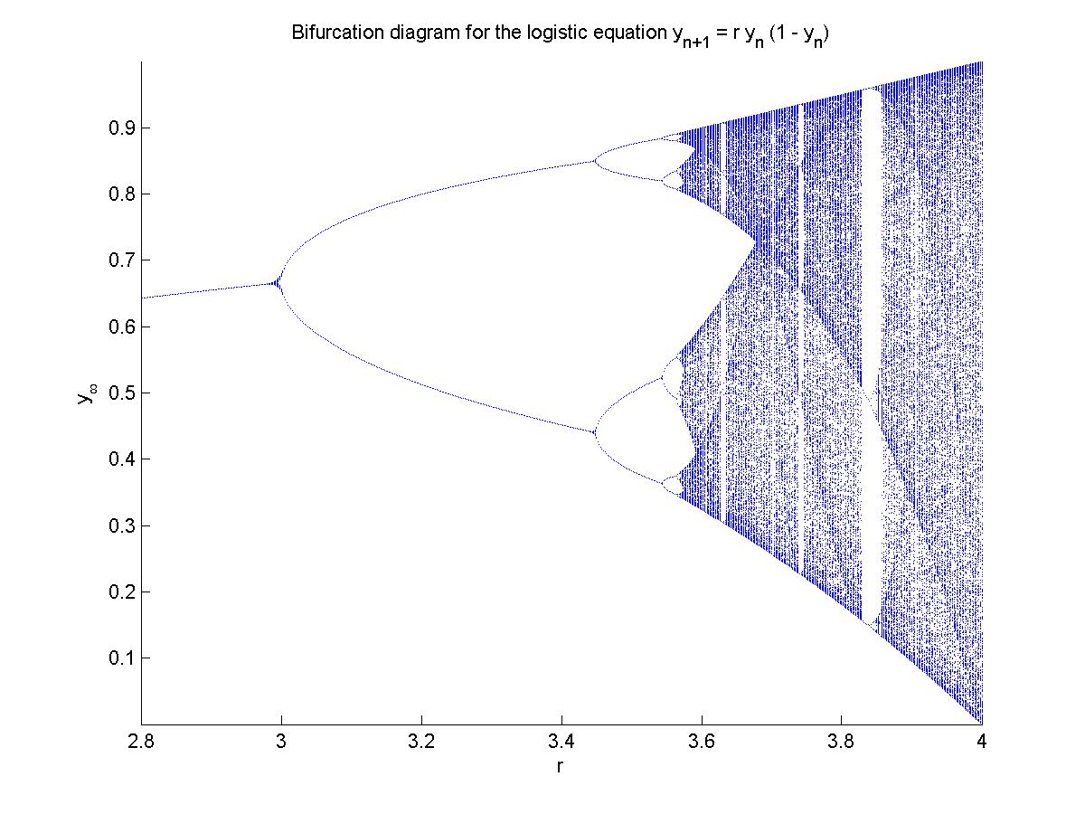
Bifurcation diagram for the logistic equation: yn+1 = r yn (1 - yn) (JPEG file) |
|
Mar 30 |
Root-finding (Word doc file) |
|
Apr 20 |
This MontyHall function performs a Monte-Carlo simulation to determine the probability of winning in the Monty Hall game,
given the two different strategies. To determine the win probability for the keep strategy, execute MontyHall(1);
compare this with the win probability for the switch strategy, by executing MontyHall(0) |