Landau-Lifshitz Equation:
time evolution of ferromagnetic materials

Consider an elementary ferromagnet which has an average magnetic moment, for example, a small sphere of iron, fixed in space. When immersed in an external magnetic field (H), the sample's magnetic moment (M) will dynamically reorient according to the Landau-Lifshitz equations. One observes both a circular precession about the magnetic field axis, and energy losses which dampen the motion until the spin comes into alignment with the magnetic field. In a real material, this realignment process occurs on the order of nanoseconds.

European call options are contracts that give the holder the right to purchase a stock at an agreed upon expiration date, at a pre-agreed upon price, called the "strike price" K. An investor can profit from holding a call option, if the stock price, S, is greater than the strike at expiry.

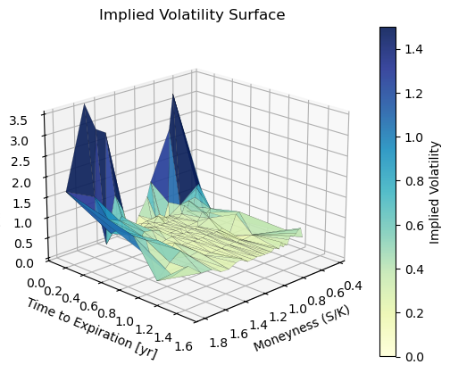
What you see pictured here is the calculated implied volatility, (often denoted, σ) of the general mills stock. Observe, for a slice of constant T, we have the characteristic U-shaped "volatility smile" in the M=S/K variable. In the flatter regions, around T≥0.8, local hills and spikes are considered points of interest, and may be targets for investigation of mispriced options.

This study is carried out on an options chain declared on General Mills (ticker symbol GIS). You can immediately view a table of all such options being traded on the market on yahoo finance.

Volatility is a tricky component which is part of a simplified model that treats the stock price as a compound brownian motion process. It is therefore not an observable quantity, and in practice a stock will not obey this drift-diffusion behavior over long periods of time. We can, however, estimate a meaningful value by solving the Black-Scholes formula numerically for the unknown σ. This framework essentially treats the prices C as market signals which implicitly reveal the opinions of traders as to the volatility of the underlying stock. Our solution will find strongly varying values of σ for each option, which we refer to as "implied volatility". Assigning a volatility to each option seems counterintuitive since we discussed that volatility is rather a property of the underlying asset. However, it also signals how much the market price of the option is deviating from that of Black-Scholes. We also find that market demand drives up both the price and the volatility. Implied volatility is an important metric for hedge funds who desire to profit from irregularly priced options.

View my calculations in detail,
download my python codes here.

Pictured is a numerical simulation of maxwells equations in a mixed vacuum / solid dielectric system which I developed in MATLAB. This demonstrates some basic optics, like reflection and refraction of the wave into the slower dielectric material.

Since optics problems like this are so diverse, and subject to innumerable instances, one would have to spend hours on modifications of the base methods, just to solve a very similar optics problem. The solution is one of software engineering rather than physics, you need a code base that takes advantage of commonalities among all conceivable applications. Here I backend all the vector calculus into simple macros and do the same with the solid geometry, so that a user doesn't need to think about it. I can then develop a simulation environment as a class in and of itself, with its time evolution, and plotting routines stored as internal methods. Call it a “C++ inspired” implementation. This object-oriented approach makes the codebase lightweight, customizable, and user friendly. It anticipates the needs of a beginning user, as it is you need only a few lines of code to produce basic scripts and solutions. Furthermore, it’s such that a more advanced user can add functionality to it without breaking the old methods.

Try it out on my GitHub.

Nonlinear Schroedinger Equation

The nonlinear schroedinger equation is related to shallow water waves, and is thought to be important for the study of rogue waves Despite its name, it does not serve any model for quantum physics.

Sports Ranking and Forecasting

The Colley Matrix Method

How can one objectively measure performance? This is Wesley Colley's method for ranking sports teams against one another. I once tried to use this in a limited way to predict the outcome of the 2014 world cup using data from friendlies and preliminary matches. My prediction had Argentina winning the tournament, though we would later find them eliminated in the final. I programmed it more extensively to rank teams from March Madness 2017 in the example pictured to the left.

The method is bias free, prefiguring the average rating to be 1/2. It is designed to only use very limited information about the teams, just their wins and losses. The method derives a matrix of interactions between the teams in order to rank all of them simultaneously by solving a linear system. Therefore, teams which never played eachother can still be ranked against one another by way of comparison to their common opponents. This enables the analysis of tournaments with a limited number of games.

For more details on the Colley method see Here to Download Colley's Original Paper.

Download my MATLAB code and data

Traveling Wave

Viscous Burgers Equation

The Viscous Burgers Equation is one of the simplest nonlinear advection diffusion equations. Analytical solutions exist via the Cole-Hopf transformation. Interestingly, it is known to admit a simple traveling wave solution under certain conditions. Pictured right, numerical solution of the traveling wave via explicit forward-Euler method.
Download my MATLAB code

Shock Wave and Solution Breakdown in Finite Time

Inviscid Burgers Equation

The Inviscid Burgers Equation enables the formation of "Shockwaves" due to its lack of any diffusion terms. For certain initial conditions the waveform will develop a steep gradient which appears to want to tumble over itself. After formation of the shock, numerical solutions breakdown entirely, and analytic solutions (if they are avaliable) are considered invalid after the time of shock formation.
Pictured right, shockwave formation and solution breakdown, numerical solutions using 3 different orders of Adams-Bashfourth methods

Mandelbrot Set

Zooming in on Mandelbrot set