Home MATH 112 Simulation Gallery

Home MATH 112 Simulation Gallery

Simulation Gallery

Evaluations and Metrics on Derivative Financial Assets

Implied Volatility of European Call Options

This study is carried out on an options chain declared on General Mills (ticker symbol GIS). You can immediately view a table of all such options being traded on the market on yahoo finance.

Volatility is a tricky component which is part of a simplified model that treats the stock price as a compound brownian motion process. It is therefore not an observable quantity, and in practice a stock will not obey this drift-diffusion behavior over long periods of time. We can, however, estimate a meaningful value by solving the Black-Scholes formula numerically for the unknown σ. This framework essentially treats the prices C as market signals which implicitly reveal the opinions of traders as to the volatility of the underlying stock. Our solution will find strongly varying values of σ for each option, which we refer to as "implied volatility". Assigning a volatility to each option seems counterintuitive since we discussed that volatility is rather a property of the underlying asset. However, it also signals how much the market price of the option is deviating from that of Black-Scholes. We also find that market demand drives up both the price and the volatility. Implied volatility is an important metric for hedge funds who desire to profit from irregularly priced options.

download my python codes here.

Implied Volatility Surfaces from Call Options data

Overview

We demonstrate some rudimentary techniques in analysis, and modeling of derivative assets, namely call options. The primary themes of the study are: Quantitative Modeling, Black-Scholes Formula, Data Mining, Data Cleaning, Numerical Methods, Regression.

Our objective is to directly calculate the implied volatility of a stock price from observing the pricing of its derivative call options. We'll numerically solve this value from the Black-Scholes Formula for a series of suitable call options on General Mills stock. The volatility thus predicted is not a constant value, but varies significantly with the option's moneyness, $M$, and time to expiration, $T$. Over these abscissae it produces a characteristic "smile" shape on a surface.

European Call Options

European call options are contracts that give the holder the right to purchase a stock at an agreed upon expiration date, at a pre-agreed upon price, called the "strike price" $K$. An investor can profit from holding a call option, if the stock price, $S$, is greater than the strike at expiry. This is said to be "in-the-money", $\frac{S}{K} = M > 1$. Otherwise, the option is worthless, since you may as well buy the stock for its market price, in this case it is said to be "out-of-the-money", $M<1$. The obvious question follows, how to price this call option on the market, taking into account all its possible payouts. We will discuss the Black-Scholes Formula below which provides an arbitrage free estimate of the call's market price, $C$.

System Data, Cleaning, and Considerations for Implied Volatility

This study is carried out on an options chain declared on General Mills (ticker symbol GIS). You can immediately view a table of all such options being traded on the market on yahoo finance. We can implement a few basic utilities from the yfinance package by Ran Aroussi to pull real time stock and options data directly into pandas DataFrames.

From experimentation, not all options on the list are compatible with the Black-Scholes model in this study, the data may be faulty because there are some contracts which are simply not being traded or are otherwise regarded as completely worthless. Others still are priced outside the admissible interval given by Black-Scholes, in which case solving for volatility will return $\pm \infty$ or other nonsense.

Yahoo Finance already tabulates their estimate for implied volatility, which provides a benchmark by which to examine our results. As yahoo finance will no doubt be using some more sophisticated models than we have for this study. We therefore need not seek numerical agreement with yahoo finance listed implied volatility, but rather we would like to observe the same qualitative behavior in our study. In the final results below you will see both a surface for our computed volatilities and those tabulated on yahoo finance.

# !pip install yfinance

import pandas as pd
import numpy as np

from scipy.stats import norm 
import yfinance as yf

# --- My Programs ---------------------------------------------
# import BlackScholesFunctions as BSF
# from BlackScholesFunctions import solve_for_iv
# from OptionsScraper import download_options_chaioptionn, todays_price #-- utilities from the yfinance package by Ran Aroussi
# -------------------------------------------------------------

from matplotlib import pyplot as plt

def download_options_chain(symbol):
    
    tk = yf.Ticker(symbol)
    # Expiration dates
    exps = tk.options

    # Get options for each expiration
    options = pd.DataFrame()
    for e in exps:
        opt_e = tk.option_chain(e)
        tempframe = pd.concat( [opt_e.calls, opt_e.puts ] )
        tempframe['expirationDate'] = e
        options = pd.concat( [options, tempframe], ignore_index=True)

    # Bizarre error in yfinance that gives the wrong expiration date
    # Add 1 day to get the correct expiration date
    options['expirationDate'] = pd.to_datetime(options['expirationDate']) + pd.Timedelta(days = 1)
    options['dte'] = options['expirationDate'].map( lambda x: (x - pd.Timestamp.today()).days / 365 )
    
    # Boolean column if the option is a CALL
    options['CALL'] = options['contractSymbol'].str[4:].apply(
        lambda x: "C" in x)
    
    options[['bid', 'ask', 'strike']] = options[['bid', 'ask', 'strike']].apply(pd.to_numeric)
    options['mark'] = (options['bid'] + options['ask']) / 2 # Calculate the midpoint of the bid-ask
    
    # Drop unnecessary and meaningless columns
    options = options.drop(columns = ['contractSize', 'currency', 'change', 'percentChange', 'lastTradeDate', 'lastPrice'])

    return options

def todays_price( symbol ):
    # for example just take the open price 
    tk = yf.Ticker(symbol)
    stockprice = tk.info['open']
    return stockprice

now import and filter the table of values appropriately:

1. only call options, (remove puts)
2. remove the options noone is trading on
3. remove the options having $C>S$, as they will have no solution in B-S formula

symbol = "GIS"
stock_price = todays_price(symbol)
dividend_rate = 0.04 #< do we want to set a value for this?

df = download_options_chain(symbol)    

# Only analyze the call options
df.drop(df[df.CALL==False].index, inplace=True)

# # Remove options with moneyness > 3.5
# df.drop(df[stock_price/df.strike > 3.5].index, inplace=True)

# # Remove options priced too low
price_lower_threshold = 0.05
df.drop(df[df.mark < price_lower_threshold].index, inplace=True)

# # See to it we remove list items which are outside the analytical bounds of the model
X = (df.mark > stock_price)

#Reset indicies in order
df.reset_index( drop=True, inplace=True )

Reading this table

• strike: as above, $K$, the price at which the option holder may choose to buy the stock at expiration
• bid: the most recent bid from a buyer
• ask: the most recent ask from a seller
• volume: quantity of this option traded in a period
• impliedVolatility: as above, the volatility implied by the option price
• expirationDate: when the option holder may exercise
• dte: time until experation in years, $T$
• mark: market price, $C$, we use this in our calculation

print("todays date is", pd.Timestamp.today())
print("todays price of", symbol,"is $", stock_price)
print("no. options in chain: ",df.shape[0])
print("")
#df.sort_values(by='mark').head(23)
df.head(15)

todays date is 2025-10-13 17:53:20.980839
todays price of GIS is $ 49.05
no. options in chain:  179

	contractSymbol	strike	bid	ask	volume	openInterest	impliedVolatility	inTheMoney	expirationDate	dte	CALL	mark
0	GIS251017C00032500	32.5	15.20	17.50	2.0	NaN	2.775394	True	2025-10-18	0.010959	True	16.350
1	GIS251017C00035000	35.0	12.90	14.80	2.0	1.0	2.367192	True	2025-10-18	0.010959	True	13.850
2	GIS251017C00037500	37.5	10.40	12.60	3.0	3.0	2.109380	True	2025-10-18	0.010959	True	11.500
3	GIS251017C00040000	40.0	8.10	9.30	1.0	5.0	1.478518	True	2025-10-18	0.010959	True	8.700
4	GIS251017C00042500	42.5	3.90	5.90	1.0	2.0	0.875001	True	2025-10-18	0.010959	True	4.900
5	GIS251017C00045000	45.0	3.20	3.60	18.0	19.0	0.568364	True	2025-10-18	0.010959	True	3.400
6	GIS251017C00047500	47.5	1.05	1.25	238.0	64.0	0.397467	True	2025-10-18	0.010959	True	1.150
7	GIS251017C00050000	50.0	0.20	0.25	1550.0	6974.0	0.385748	False	2025-10-18	0.010959	True	0.225
8	GIS251017C00055000	55.0	0.00	0.10	14.0	4149.0	0.621098	False	2025-10-18	0.010959	True	0.050
9	GIS251017C00057500	57.5	0.00	0.20	1.0	1254.0	0.890626	False	2025-10-18	0.010959	True	0.100
10	GIS251017C00075000	75.0	0.00	0.20	1.0	54.0	1.859376	False	2025-10-18	0.010959	True	0.100
11	GIS251017C00080000	80.0	0.00	0.60	3.0	6.0	2.496098	False	2025-10-18	0.010959	True	0.300
12	GIS251121C00027500	27.5	19.00	22.90	75.0	0.0	1.062505	True	2025-11-22	0.106849	True	20.950
13	GIS251121C00032500	32.5	14.10	18.00	3.0	5.0	0.845705	True	2025-11-22	0.106849	True	16.050
14	GIS251121C00035000	35.0	12.10	14.00	NaN	6.0	0.888673	True	2025-11-22	0.106849	True	13.050

The Black-Scholes Formula

The call option price is given, according to the model, as

\begin{equation} C(S,T) = S e^{-qT} N(d_1) - K e^{-rT} N(d_2) , \end{equation}

where $N(x)= \frac{ 1 }{ \sqrt{2 \pi} } \int_{-\infty}^{x} e^{-\frac{z^2}{2} } \ dz $ is the cumulative distribution function of the standard normal, and

\begin{align} d_1 &= \frac{\log\left(\frac{S}{K}\right) + \left(r-q+\frac{\sigma^2}{2} \right) T }{\sigma \sqrt{T}} , \\ d_2 &= d_1 - \sigma\sqrt{T} . \end{align}

Here we have several variables and model parameters, most of which are, in principle, very easy to estimate.

• $C$ : Call option price
• $S$ : Price of underlying asset
• $K$ : Strike
• $q$ : Dividend rate of underlying asset
• $r$ : Characteristic risk-free interest rate
• $T$ : Time to expiration
• $\sigma$ : volatility

Volatility vs Implied Volatility

Volatility is a tricky component which is part of a simplified model that treats the stock price as a compound brownian motion process. It is therefore not an observable quantity, and in practice a stock will not obey this drift-diffusion behavior over long periods of time. We can, however, estimate a meaningful value by solving the Black-Scholes formula numerically for the unknown $\sigma$. This framework essentially treats the prices $C$ as market signals which implicitly reveal the opinions of traders as to the volatility of the underlying stock.

Our solution will find strongly varying values of $\sigma$ for each option, which we refer to as "implied volatility". Assigning a volatility to each option seems counterintuitive since we discussed that volatility is rather a property of the underlying asset. However, it also signals how much the market price of the option is deviating from that of Black-Scholes. We also find that market demand drives up both the price and the volatility. Implied volatility is an important metric for hedge funds who desire to profit from irregularly priced options.

Analytical Consequences of the B-S formula

The following can be easily proved using only differential calculus, and give certain expectations for the behavior of $C$ and $\sigma$ and the subsequent numerical solution.

• a sufficient condition for the monotonicity of $C$ is if the following holds, $ \sigma^2 > \frac{2\log\left(\frac{S}{K}\right)}{T} + 2(r-q)$, in which case $C$ is guaranteed to be strictly increasing with $\sigma$. Corroborating our expectation that higher market prices will necessarily be on those options with higher implied volatility.

Let $\tilde{S} = S e^{-qT}$ and $\tilde{K} = K e^{-rT}$,

• if the option is in-the-money, $S>K$, the following hold
  1. the price is bounded from above and below, $ \tilde{S}-\tilde{K} \leq C(S,T) \leq \tilde{S}$
  2. furthermore, as $\sigma \rightarrow 0$ we have $C(S,T) \rightarrow \tilde{S}-\tilde{K}$
  3. in the other direction, $\sigma \rightarrow \infty$ implies $C(S,T) \rightarrow \tilde{S}$
• if the option is out-of-the-money, $S<K$, the following hold
  1. the price is bounded from above and below, $ 0\leq C(S,T) \leq \tilde{S}$
  2. furthermore, as $\sigma \rightarrow 0$ we have $C(S,T) \rightarrow 0$, and this option is clearly worthless without any volatility to gamble on.
  3. in the other direction, $\sigma \rightarrow \infty$ implies $C(S,T) \rightarrow \tilde{S}$
• These facts together reproduce the time-boundary conditions of the Black-Scholes model: at expiration $ C(S,0) = \max\{ 0, S-K \}$

Solution Technique

We solve for the value of $\sigma$ which makes the output of the Black-Scholes formula match the market price from data. We estimate $\sigma$ numerically using newtons method, and a hybrid implementation of the bisection method to overcome overshooting from newtons method. This does however lead to a downside where one has to filter out deficient results that run away to infinity.

#------------------------------------------------------------
def call_option_price( S, K, T, r, sigma, q=0 ):
    if T==0:
        C = max(S-K,0)
        return C
    if sigma == 0:
        C = max( S * np.exp(-q*T) - K *np.exp(-r*T) , 0 )
        return C 
    
    d1 =( np.log(S/K) + ( r - q + 0.5 * sigma**2 ) * T )/( sigma*np.sqrt(T) ) 
    d2 = d1 - sigma*np.sqrt(T)
    
    C = S * np.exp(-q*T) * norm.cdf( d1, 0,1 ) - K *np.exp(-r*T) * norm.cdf( d2, 0, 1 )
        
    return C
#------------------------------------------------------------

#------------------------------------------------------------
def loss_fn( C, S, K, T, r, sigma, q=0 ):
    return  call_option_price( S, K, T, r, sigma, q) - C  

def loss_grad_fn( C, S, K, T, r, sigma, q=0,  epsilon=0.0005):
    f = lambda ss: loss_fn( C, S, K, T, r, ss, q )
    return ( f(sigma+epsilon) - f(sigma) )/( epsilon )
#------------------------------------------------------------

#------------------------------------------------------------
def solve_for_iv( C, S, K, T, r, sigma_guess=1.0, Niter=20, ftolerance=0.0005, q=0, verbose=False   ):
    
    if T==0:
        converged = True
        return np.nan
    
    converged = False
    sigma = sigma_guess
    
    f  = lambda sig: loss_fn(      C, S, K, T, r, sig, q=q)
    df = lambda sig: loss_grad_fn( C, S, K, T, r, sig, q=q)
    
    # compute with newtons method
    for n in range(Niter):
        
        loss = f( sigma )
        
        if verbose:
            print("Itr ", n, ", f_loss =", loss, ", sigma = ", sigma )
            
        if abs(loss)<ftolerance:
            converged = True
            if verbose:
                print("Converged!")
            break
                
        else:
            loss_grad = df( sigma ) 
            
            if loss_grad == 0.0:
                # default to bisection
                if loss > 0:
                    sigma = sigma/2
                else:
                    sigma = sigma*2
            else:
                #Newton
                sigma0 = sigma - loss/loss_grad
            
            # default to bisection if falls below zero
            # or goes to infinity just double it
            if sigma0 < 0:
                sigma = sigma/2
            elif sigma0 == np.inf:
                sigma = 2*sigma
            else:
                sigma = sigma0
            
    #if converged:
    #    pass
    #else:
    #    print("did not converge in", Niter, "iterations. Final error delta_C =", loss )
        
    return sigma        
        
#------------------------------------------------------------

#------------------------------------------------------------
def show_iv_solution_on_graph(  C, S, K, T, r, sigma_soln, smax=-1, q=0  ):
    
    from matplotlib import pyplot as plt
    
    f = lambda sig: call_option_price( S, K, T, r, sig )
    
    smin = 0.0
    if smax == -1:
        smax = 100.0
        
    s = np.linspace(smin,smax,100)
    y = 0*s
    for i in range(len(s)):
        y[i] = f(s[i])

    plt.figure()
    plt.plot( s, y )
    plt.plot( [smin, smax], [C,C], '--' )
    plt.plot( sigma_soln, f(sigma_soln), 'o' )
    plt.xlabel("$\sigma$")
    plt.ylabel("$C_{BS}(\sigma)$")
    plt.legend(["$C_{BS}(\sigma)$","$C_{market}$","$\sigma_{implied}$"])
    plt.show()

# Does our method work?
# Check it agrees with the implied volatility in the dataframe

if True:
    myRow = df[df.mark > stock_price-df.strike].iloc[0]
    sigma_real = myRow["impliedVolatility"]
    S = stock_price
    K = myRow["strike"]
    T = myRow["dte"]
    r = 0.06 #some number for interest rate
    q = dividend_rate
    C = myRow["mark"]
    
    print("Example of soln for implied volatility:")
    print("  system vars: S =",S,", K =",K,", T =",T,", r =",r,",")
    print("      sigma_real =",sigma_real,", C =",C)
    print("")
    print("iteratively solve for sigma: ")
    sigma = solve_for_iv( C, S, K, T, r, sigma_guess=8.8, q = q, verbose = True )
    print("implied sigma estimated = ", sigma )
    print("final error in sigma    = ", abs( sigma-sigma_real ) )

    show_iv_solution_on_graph(  C, S, K, T, r,  sigma, q=q, smax = 6.0 )

Example of soln for implied volatility:
  system vars: S = 49.05 , K = 50.0 , T = 0.010958904109589041 , r = 0.06 ,
      sigma_real = 0.3857483300781249 , C = 0.225

iteratively solve for sigma: 
Itr  0 , f_loss = 16.877102364531797 , sigma =  8.8
Itr  1 , f_loss = 8.329040081706596 , sigma =  4.4
Itr  2 , f_loss = -0.033335146584594716 , sigma =  0.25884158062834217
Itr  3 , f_loss = 0.0005925291107825303 , sigma =  0.27943522513880337
Itr  4 , f_loss = 3.798208375316303e-07 , sigma =  0.27908164284534187
Converged!
implied sigma estimated =  0.27908164284534187
final error in sigma    =  0.10666668723278305

#
#  well, we're just gonna send it
#
S = stock_price
K = df.loc[:,"strike"].to_numpy( )
T = df.loc[:,"dte"].to_numpy( )
r = 0.07 #some number for interest rate
q = dividend_rate
C = df.loc[:,"ask"].to_numpy( )
M = S/K

sigma_implied  = np.zeros( len(K) )

for i in range( len(K) ) :
    sigma_implied[i] = solve_for_iv( C[i], S, K[i], T[i], r, q = q, sigma_guess=9.0, verbose = False )
    df.loc[i,'calculated sigma implied'] = sigma_implied[i]

df.sort_values(by='mark').head(8)

	contractSymbol	strike	bid	ask	volume	openInterest	impliedVolatility	inTheMoney	expirationDate	dte	CALL	mark	calculated sigma implied
57	GIS260116C00077500	77.5	0.00	0.10	1.0	160.0	0.449224	False	2026-01-17	0.260274	True	0.050	0.430997
8	GIS251017C00055000	55.0	0.00	0.10	14.0	4149.0	0.621098	False	2025-10-18	0.010959	True	0.050	0.703850
24	GIS251121C00060000	60.0	0.00	0.10	3.0	38.0	0.373053	False	2025-11-22	0.106849	True	0.050	0.002063
23	GIS251121C00057500	57.5	0.00	0.10	29.0	279.0	0.315437	False	2025-11-22	0.106849	True	0.050	0.287352
54	GIS260116C00070000	70.0	0.00	0.15	49.0	933.0	0.395514	False	2026-01-17	0.260274	True	0.075	0.375154
37	GIS251219C00070000	70.0	0.00	0.20	1.0	1.0	0.495122	False	2025-12-20	0.183562	True	0.100	0.472979
56	GIS260116C00075000	75.0	0.00	0.20	1.0	1222.0	0.475591	False	2026-01-17	0.260274	True	0.100	0.455315
162	GIS270115C00110000	110.0	0.05	0.15	10.0	27.0	0.340827	False	2027-01-16	1.257534	True	0.100	0.323773

# () - A quick check on my T moneyness plane

plt.figure()
plt.plot( T, M, 'o' )
plt.xlabel("Time to Expiration (yr)")
plt.ylabel("Moneyness (S/K)")
plt.title("Where does our data live in the plane?")
plt.show()


# # Uncomment this to search for extreme values of sigma_implied
#plt.figure()
#plt.plot( T, sigma_implied, 'o' )
#plt.xlabel("Time to Expiration (yr)")
#plt.ylabel("sigma implied")
#plt.title("Results of implied volatility computation")
#plt.show()

Remarks

This chart is nothing more than the data loci of our two independent variables $M=S/K$ and $T$, verifying that after all the filtering, we still have some meaningful datapoints that span the plane.

M_cutoff = 5.0
T_cutoff = 1.6
indic    = (M<M_cutoff) * (T<T_cutoff)

fig = plt.figure()
ax = fig.add_subplot( 111, projection='3d')

surf = ax.plot_trisurf( M[indic], T[indic], C[indic] 
                      , cmap="YlGnBu"
                      , antialiased=True
                      , alpha = 0.90
                      , linewidth=0.1
                      , edgecolor="k"
                      )

cbar = fig.colorbar(surf, ax=ax)
cbar.set_label("Price: C")

#ax.set_ylim([0,1])
ax.set_xlabel("Moneyness (S/K)")
ax.set_ylabel("Time to Expiration [yr]")
ax.set_zlabel("Price: C")

plt.title("Price Surface")

ax.view_init(elev=20, azim=45)

# plt.tight_layout()

plt.show()

Remarks

This chart for the option prices matches the basic shape we expect from the analytical B-S formula

#
# Surface
#

# M_cutoff = 3.3
sigma_cutoff = 5
indic2 = indic * ( sigma_implied < sigma_cutoff )

fig = plt.figure()
ax = fig.add_subplot( 111, projection='3d')

surf = ax.plot_trisurf( M[indic2], T[indic2], sigma_implied[indic2] 
                      , cmap="YlGnBu"
                      , antialiased=True
                      , vmax = 1.5
                      , alpha = 0.90
                      , linewidth=0.1
                      , edgecolor="k"
                      )

cbar = fig.colorbar(surf)
cbar.set_label("Implied Volatility")

ax.set_ylim([0,T_cutoff])
ax.set_xlabel("Moneyness (S/K)")
ax.set_ylabel("Time to Expiration [yr]")
ax.set_zlabel("Implied Volatility")

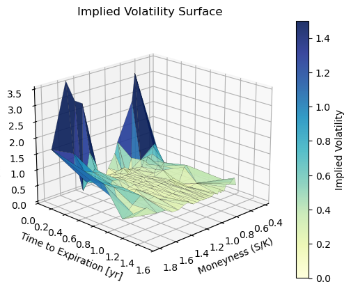
plt.title("Implied Volatility Surface")

ax.view_init(elev=20, azim=45)

# plt.tight_layout()

plt.show()

Remarks

This is the calculated implied volatility. Observe, for a slice of constant $T$, we have the characteristic U-shaped "volatility smile" in the $M=S/K$ variable. In the flatter regions, around $T \geq 0.8$, local hills and spikes are considered points of interest, and may be targets for investigation of mispriced options.

sigma_yahoofinance = df.loc[:,"impliedVolatility"]

fig = plt.figure()
ax = fig.add_subplot( 111, projection='3d')

surf = ax.plot_trisurf( M[indic2], T[indic2], sigma_yahoofinance[indic2] 
                      , cmap="YlGnBu"
                      , antialiased=True
                      , vmax = 1.5
                      , alpha = 0.90
                      , linewidth=0.1
                      , edgecolor="k"
                      )

cbar = fig.colorbar(surf)
cbar.set_label("Implied Volatility")

ax.set_ylim([0,T_cutoff])
ax.set_xlabel("Moneyness (S/K)")
ax.set_ylabel("Time to Expiration [yr]")
ax.set_zlabel("Implied Volatility")

plt.title("Implied Volatility Surface, from yahoo finance")

ax.view_init(elev=20, azim=45)

# plt.tight_layout()

plt.show()

Remarks

This is the surface for the implied volatility provided by yahoo finance data. It qualitatively matches our calculation.