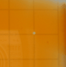
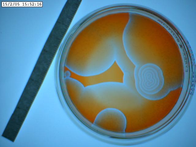
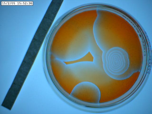
Following we see two images captured with
the iSight camera. The Petri dish was on the lightbox and what's shown below
are the best images of a sequence of a few hundred. The variation of the background
illumination due to the 60 Hz effect described above was very deleterious.
The iSight setup was abandonded after this run. One can discern spiral waves
in these images.
|
|
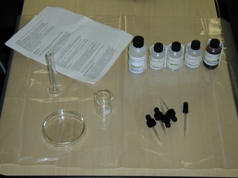
A word of caution: the Petri dish that comes with the kit is not suitable
as it has a very uneven bottom. You can see from the images above that the
center area appears more illuminated than the area close to the rim; this
is because the dish becomes shallower towards the center. We attributed the
development of patterns predominantly near the rim to this manufacturing imperfection.
We tried to create target patterns in the center of the dish but we were
not successful. Thus, the supplied Petri dish was put aside in favor of a
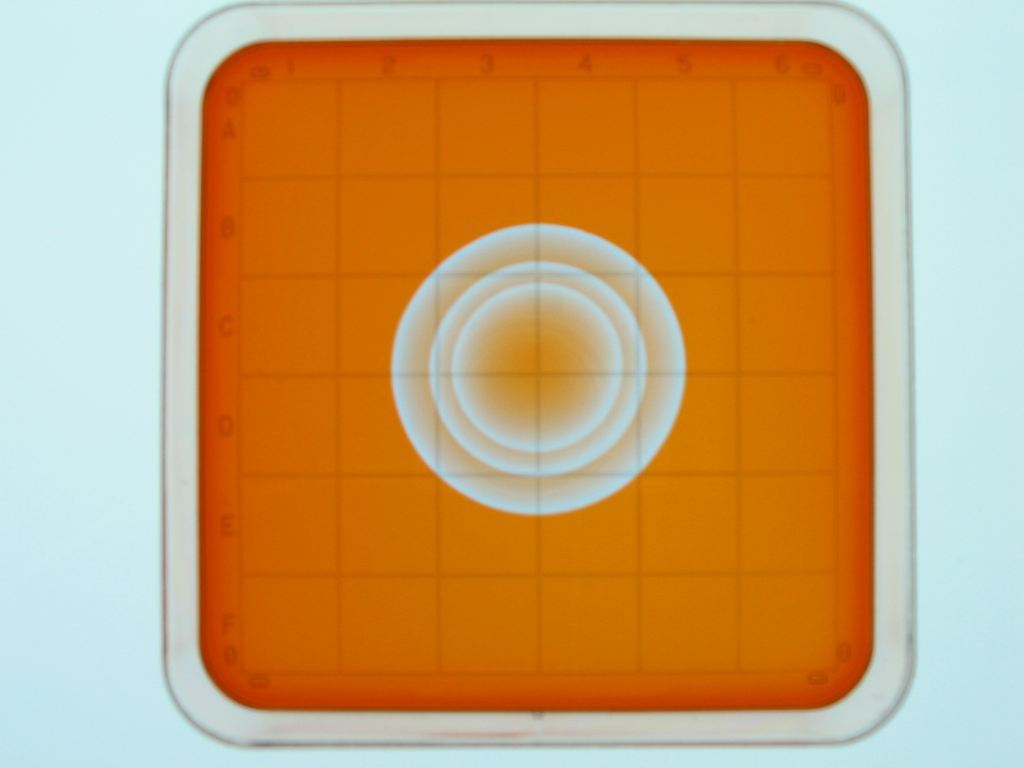
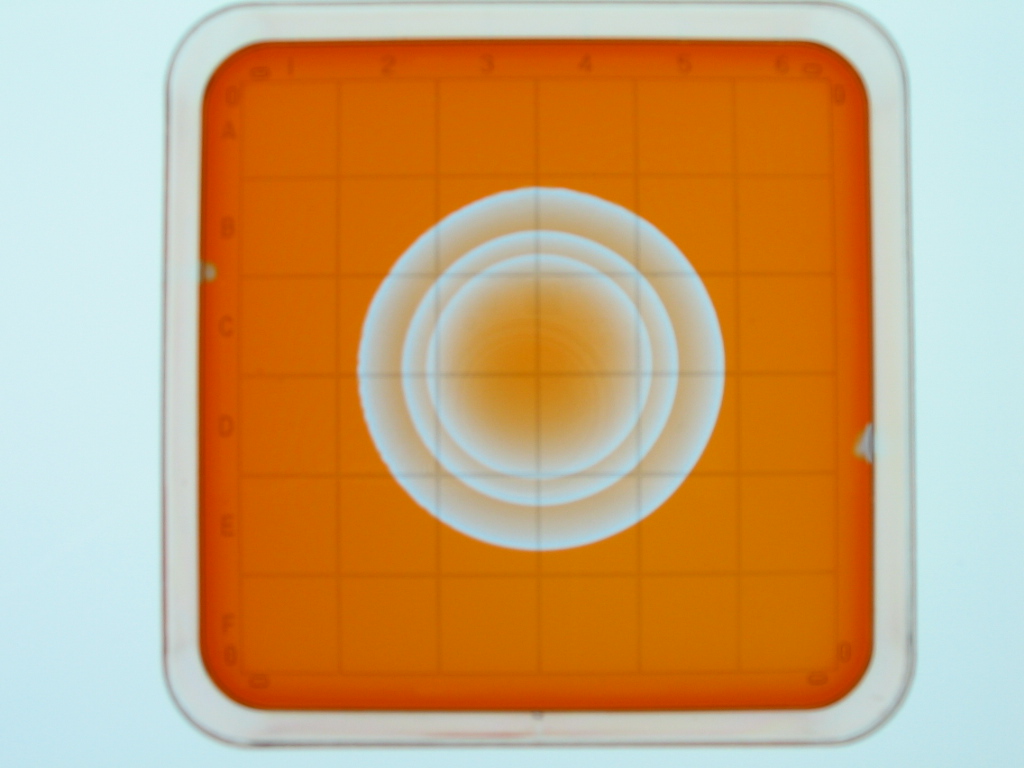
plastic square Petri dish with a perfectly flat bottom. We employed the square
Petri dish in the following way: A drop of 0.1 % solution of Triton-X was
added to the solution prior to its introduction into the dish and regular
dish soap was spread with a paper towel on the inside of the dish cover to
eliminate fogging. With this dish we have not observed any bubbles, and the
uniformity of depth keeps the solution in an excited state (red) for many
tens of seconds. The dishes have a grid etched on the outside of the bottom
hence facilitating the use of a silver wire to initiate target patterns at
the exact center of the dish. The dish being square also helps when the experiment
is simulated on a square domain with no-flux boundary conditions (makes it
easier to convince a doubting audience of the correspondence between modeling
and experiment without having to explain much). Here are two images captured
with the Canon A85; They show a pacemaker center that produced three bands
of oxidation and then died out (the group of bands then expanded out at a
constant speed with the region behind the bands returning to the reduced state):
|
|
The images above were taken 49 seconds apart.
NOTE: When the dish
cover is in place the digital camera (when set to auto-focus) likes to focus
on its reflection off the dish cover top face hence the stuff happening 4
mm below the cover tend to be out of focus; one solution is to manually focus
the camera with the cover off and then to place the cover, the other solution
is to simply not cover the dish. The following graphs show the result of post-processing
a number of images from this sequence, and from another sequence where one
band of oxidation moved out from the center which did not produce any more
waves. ImageJ was used (along with the Radial Profile plugin) to extract
information from the relevant images:
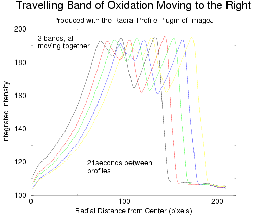
|
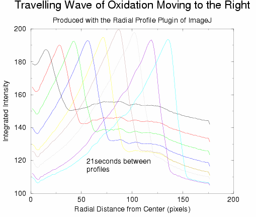
|
Obviously, the fronts move with constant speed. In both graphs above, a low
value for the integrated intensity corresponds to the red state of the solution
(reduced) while the peaks correspond to the blue state of the solution (oxidized,
see 2D images further up). In all our experiments, the mixed solution almost
always undergoes 1.5 bulk oscillations prior to being poured into the dish
(red-->blue-->red). Once in the dish, the swirling/jostling involved
in centering the dish under the camera produces another 1.5 bulk oscillations
(red-->blue-->red).
Finally, near the end of a particularly good run of target patterns appearing
all over the place, it was observed that a particular pacemaker site
dominated the whole domain (all other pacemakers disappeared). The following
animated gif file shows a bifurcation of the frequency of the pacemaker. We
have no idea how to investigate this mathematically...if you, the reader,
can help us then send us an e-mail. The following short loop is cropped out
of a larger sequence of larger-in-size images:
B) Temporal
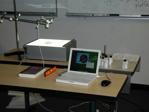
Oscillations in the Well-stirred Belousov-Zhabotinsky reaction:
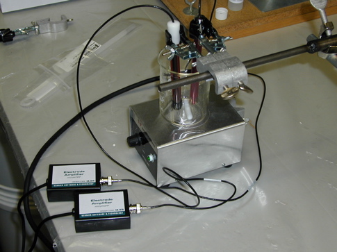
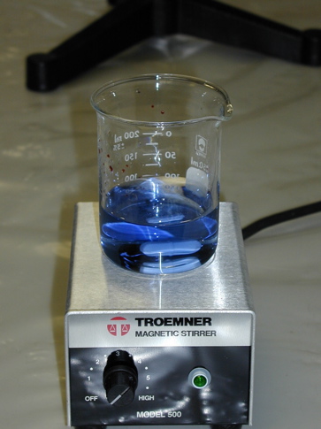
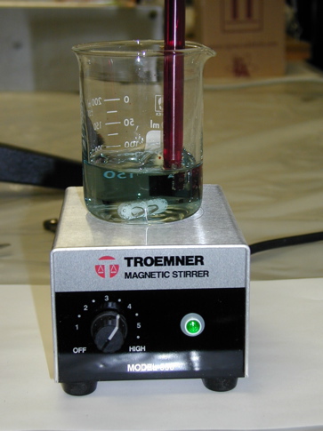
Here are some images of the setup and of the oscillations observed thus far.
In the bottom row images the time from blue to blue is about 25 seconds.
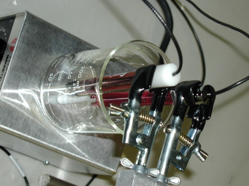
NOTE: The
Weiss Bromide-sensitive and Platinum
electrodes are connected to the Vernier
LabPro interface (not shown
in these shots) through Vernier
Electrode
Amplifiers.
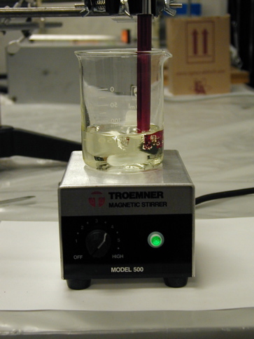
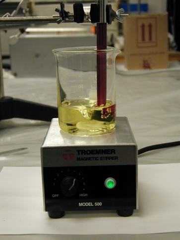
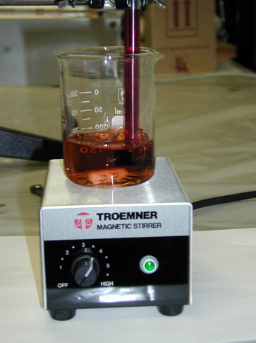
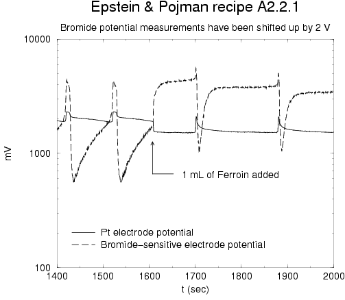
No chemical potentials were measured for the solution shown above. Below
we show some pictures of our first attempt to measure the catalyst concentration
(Pt electrode) in the well-stirred BZ reaction:
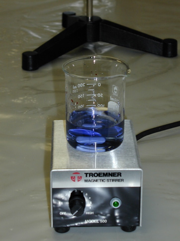
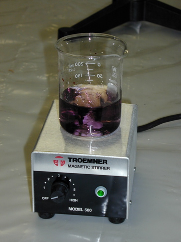
In the above 2X2 panel, the top row shows oscillations in the Cerium catalyzed
BZ reaction (color oscillates between clear and yellow); the bottom row shows
the color oscillation after adding 1 mL of Ferroin (color now oscillates between
red-brown and blue-green). The graph below shows the electrode potential
measurements before and after the addition of the Ferroin in a run with the
same recipe as in the pictures above but with the Bromide electrode present:
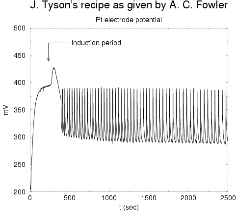
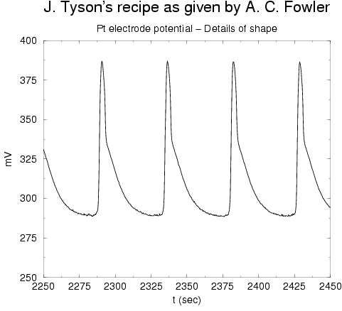
We also tried a recipe due to Tyson (no KBr used). For this one we only measured
the cerrium ions:
Numerical Simulations:
A) Pattern
Formation in the Unstirred Belousov-Zhabotinsky reaction: Coming
soon.
B) Temporal
Oscillations in the Well-stirred Belousov-Zhabotinsky reaction: Coming
soon.