MMFit  Software

DOWNLOAD  ZIP for  MATLAB-based Program  MMFit_BULK

 

Muller Matrix Ellipsometer Project

For data analysis measured

at  U4IR beamline NSLS-BNL

Send a request for MATLAB-based Program  MMFit_FILMS

 

DOWNLOAD  ZIP  with MATLAB Functions T_ij (4x4) for your own software development

 

DOWNLOAD    PDF  Method description  written by Roman Basistyy as a part of his PhD Theses, 2014

MANUAL  for  MMFit_BULK  fitting Program

 

Bulk material can contain any combinations of electric, magnetic, magneto-electric and chiral oscillations. SHO model and Berreman formalism were utilized to get representation of pseudo-dielectric <> function, ellipsometricreflectance, transmittance and Mueller matrices. Maximum number of oscillators in this version is 36 which can be increased if needed. Levenberg-Marquardt algorithm was used for fitting, where number of iterations changing is available for user.

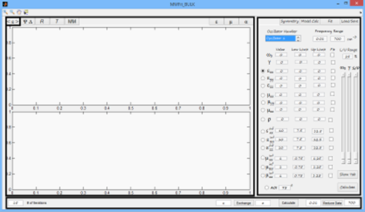
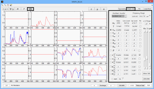
             Figure 1 Start window of MMFit program. By default data panel (left) is for pseudo-dielectric function and model panel (right) is for model creation (“Model Calc”).

Program consists of three main panels. Left one, consisting of eight subpanels,  is for data and models representation, right one, consisting from four to five subpanels in different versions, is for loading, saving data and models, adjusting fitting parameters, creation of models, choosing tensor symmetry. Low panel allows to adjust data (reduce to desirable range), choose number of iterations for fitting, calculate current model and exchange columns in current model (analog to Euler rotation by 90 degrees in any direction).

 

1. Working with Data

In order to load or save data and models one should click on “Load/Save” button in right panel.            

             Figure 2 Load/Save panel in MMFit program after loading mmd format file and clicking on “MM Panel” button, containing three Mueller matrix components (m₂₁,m₃₃,m₃₄). Blue line – data. Red line – model.

 

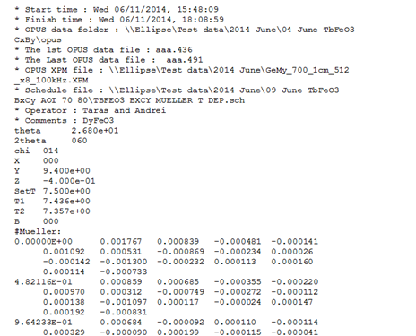
There are 17 buttons on “Load/Save” panel. “Load *.mmd Data” allows user to load Mueller matrices data in mmd format. There are 16 non-normalized columns in mmd data file. MMFit normalize all MM components to the first MM component.

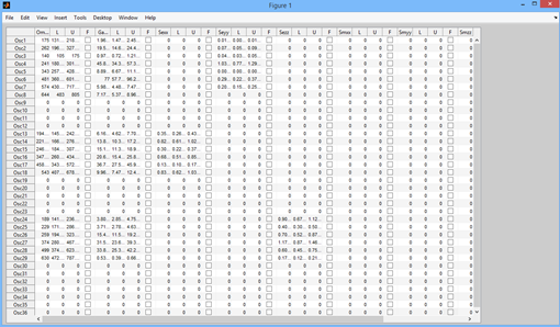
                    Figure 3 MMD data file structure.

 

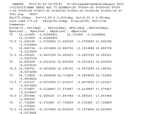
“Load *.epd Data” button allows user to load data in epd format, containing real part of pseudo-dielectric function (column six), imaginary part of pseudo-dielectric function (column seven), function (column two) ,function (column three) . Mmd and epd data formats are shown in Figures 6.3,6.4 correspondingly.

            

                    Figure 4 EPD data file structure.

Following twelve buttons allow user to load separately pseudo-dielectric function data, function data, function data, reflection data, transmission data. Data files must contain two columns only without any headers. First column should be frequency in inverse centimeters, second column is intensity data. If one loads pseudo-dielectric function data using  “Load *.epd Data” and then load another pseudo-dielectric function data using “Load <Eps1> Data” and/or “Load <Eps2> Data”, corresponding data will be rewritten to the newest one. This works for andfunctions data as well.

“Reduce Data” button on the lower panel allows to cut data in the defined by user range”. To restore data original data file should be loaded and reduced data will be rewritten to the new one.

“Load Project” button allows to load project previously saved by “Save Project” button. “Save Project” button gives overall saving option: all available data, models and parameters will be recorded.

“Save FitData” button saves all models and all data to separate files, consisting of two columns: first one is frequency, second one is intensity. If there were no loaded data previously, MMFit programs provides file with zero data. The same is valid for models. Total number of files saved after “Save FitData” button clicked is 25.

2 Working with Models

For creation and modifying model function user should click on “Model Calc” button in the right panel.            

                    Figure 5      “Model Calc” panel with “MM” data panel after creating rough starting model for fitting. Blue line – data. Red line – model.

 

There are three sliders available for adjusting different values. First slider (from the left to the right) always changes oscillation frequency value. Second slider always changes Gamma (broadening coefficient) value. Third slider changes value chosen by radiobuttons. When one changes values with sliders current models are redrawn dynamically. Main purpose of this visualization is to find starting fitting point maximally close to the original data.

 

Figure 6 “Show Tab” panel view with model parameters.

 

“Show Tab” button draws additional panel which gives overall picture of the current model. User has option to change available values from this panel as well. After adjusting all values additional click on free space should be made and current window should be closed. “L” stands for low fitting boundary. “U” stands for high fitting boundary. “F” stands for fit. If some value is supposed to be fitted, one should mark corresponding checkbox. When checkbox is chosen, “L” and ”U” values are updated automatically by value from “L/U Range” edit field percent from the initial value of current parameter.

“Fitting Range” allows to choose appropriate range in inverse centimeters for fitting.

In order to choose ME tensor symmetry or add off diagonal components of electric permittivity tensor user should click on “Symmetry” button in the right panel.

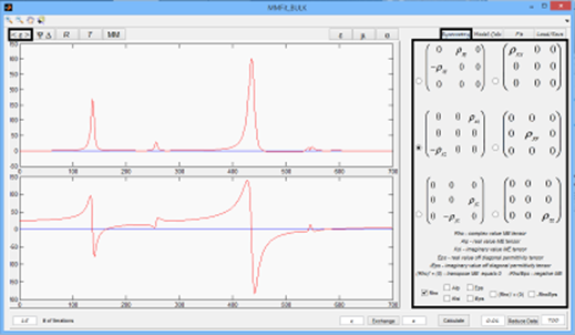
             Figure 7 “Symmetry” panel view and pseudo-dielectric function data panel with model containing ME oscillator at 545 cm^-1.

 

There are six available options to construct ME tensor which are shown in Figure 6.7. Checkboxes in the low part of the panel allows to choose different options for ME tensor. “Rho” checkbox makes component of ME tensor complex , “Alp” checkbox makes them real, “Ksi” checkbox makes them purely imaginary, “Eps” makes ME tensor 0 and add corresponding real components to electric permittivity tensor. It should be noted that for this choice only off diagonal components available.”iEps” does the same as  “Eps” but makes components purely imaginary.”Rho’ = 0” make transpose ME tensor 0 and “-Rho/Eps” makes negative ME tensor or if “Eps”, “iEps” options are chosen makes negative off diagonal terms of permittivity tensor.

After model is constructed clicking on “Calculate ” button plots model in the left panel for all functions. There is “Calculate ” button on the lower panel and on the “Model Calc” panel as well.

 

3 Fitting

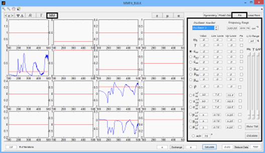
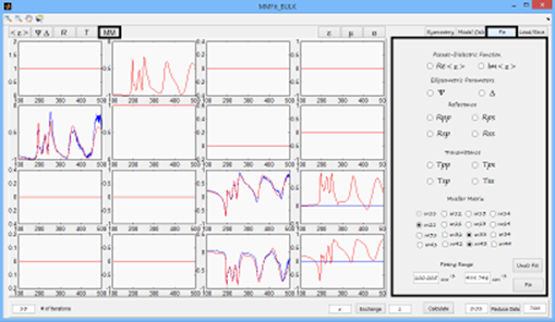
             Figure 8 “Fitting” panel view with “MM” data panel after fitting three Mueller matrix components. Blue line – data. Red line – model.

 

“Fit” panel allows to choose different set of data for simultaneous fitting. Desired data for fit should be marked by means of radio buttons. After choosing appropriate sets of data fitting frequency boundaries could be adjusted in “Fitting range Field”.”Fit” button starts fitting procedure. After fit is finished, fitted values are renewed. Left edit box in the low panel allows to adjust number of fitting iterations.