Go to ECE489 Experiment | 1 | 2 | 3 | 4 | 5 | 6 | 7 | 8 | 10 | 11 | 12 | 13 | 14 | ECE Lab home
![]()
|
|
Go to ECE489 Experiment | 1 | 2 | 3 | 4 | 5 | 6 | 7 | 8 | 10 | 11 | 12 | 13 | 14 | ECE Lab home |
|
ECE 489 Communications Systems Laboratory
Experiment 9 : THE NOISE CHANNEL MODEL
ACHIEVEMENTS:
Definition of the macro CHANNEL
MODEL module. Ability to set up a noisy band limited channel for subsequent
experiments; measurement of filter characteristics,. measurement of signal-to-noise
ratio with the WIDEBAND TRUE RMS METER. Observation of different levels of signal-to-noise
ratio with speech.
PREREQUISITES: None
EXTRA MODULES: WIDEBAND TRUE RMS METER, NOISE GENERATOR, BASEBAND CHANNEL
FILTERS module; 100 kHz CHANNEL FILTERS module optional
Since TIMS is about modelling communication systems it
is not surprising that it can model a communications channel.
Two types of channels are frequently required, namely low pass and bandpass.
LOWPASS (OR BASEBAND) CHANNELS
A lowpass channel by definition should have a bandwidth
extending from DC to some upper frequency limit. Thus it would have the characteristics
of a lowpass filter .
A speech channel is often referred to as a lowpass channel, although it does
not necessarily extend down to DC. More commonly it is called a baseband
channel.
A bandpass channel by definition should have a bandwidth covering a range of frequencies not including DC. Thus it would have the characteristics of a bandpass filter.
Typically its bandwidth is often much less than an octave, but this restriction is not mandatory. Such a channel has been called narrow band.
Strictly an analog voice channel is a bandpass channel,
rather than lowpass, as suggested above, since it does not extend down to DC.
So the distinction between baseband and bandpass channels can be blurred on
occasion.
Designers of active circuits often prefer bandpass channels, since there is
no need to be concerned with the minimization of DC offsets.
For more information refer to the chapter entitled Introduction to modelling with TIMS, within Volume A1 -Fundamental Analog Experiments, in the section entitled 'bandwidths and spectra'.
The above description is an oversimplification of a practical system. It has concentrated all the bandlimiting in the channel, and introduced no intentional pulse shaping. In practice the bandlimiting, and pulse shaping, is distributed between filters in the transmitter and the receiver, and the channel itself. The transmitter and receiver filters are designed, knowing the characteristics of the channel. The signal reaches the detector having the desired characteristics.
Whole books have been written about the analysis, measurement, and optimization of signal-to-noise ratio (SNR).
SNR is usually quoted as a power ratio, expressed in decibels. But remember the measuring instrument in this experiment is an rms voltmeter, not a power meter. See Tutorial Question Q6.
Although, in a measurement situation, it is the magnitude of the ratio S/N
which is commonly sought, it is more often the
![]() which is available. In other words,
in a non-laboratory environment, if the signal is present then so is the
noise; the signal is not available alone.
which is available. In other words,
in a non-laboratory environment, if the signal is present then so is the
noise; the signal is not available alone.
In this, and most other laboratory environments, the noise is under our control,
and can be removed if necessary. So that
![]() rather than
rather than ![]() can be measured directly.
can be measured directly.
For high SNRs there is little difference between the two measures.
A representative noisy, bandlimited channel model is shown in block diagram form in Figure 1 of the following page.
Band limitation is implemented by any appropriate filter.
The noise is added before the filter so that it becomes bandlimited by the same filter that band limits the signal. If this is not acceptable then the adder can be moved to the output of the filter, or perhaps the noise can have its own bandlimiting filter.
 |
| Figure 1: channel model block diagram |
Controllable amounts of random noise, from the noise source, can be inserted into the channel model, using the calibrated attenuator. This is non signal-dependent noise.
For lowpass channels lowpass filters are used.
For bandpass channels bandpass filters are used.
Signal dependent noise is typically introduced by channel non-linearities, and includes intermodulation noise between different signals sharing the channel (cross talk). Unless expressly stated otherwise, in TIMS experiments signal dependent noise is considered negligible. That is, the systems must be operated under linear conditions. An exception is examined in the experiment entitled Amplifier overload (within Volume A2 -Further & Advanced Analog Experiments).
In patching diagrams, if it is necessary to save space, the noisy channel will be represented by the block illustrated in Figure 2 below. Color may vary
 |
| Figure 2: the macro CHANNEL MODEL module |
Note it is illustrated as a channel model module. Please do not look for a physical TIMS module when patching up a system with this macro module included. This macro module is modelled with five real TIMS modules, namely:
An INPUT ADDER module.
A NOISE GENERATOR module.
A bandlimiting module. For example, it could be:
Any single filter module;
such as a TUNEABLE LPF (for a baseband channel).
A BASEBAND CHANNEL FILTERS module, in which
case it contains three filters, as well as a direct through connection.
Any of these four paths may be selected by a front panel
switch. Each path has a gain of unity. This module can be used
in a baseband channel. The filters all have the same slot bandwidth
(40 dB at 4 kHz), but differing passband
widths and phase characteristics.
A 100 kHz CHANNEL FILTERS module, in which case it contains
two filters, as well as a direct through connection. Any of these three
paths may be selected by a front panel switch. Each path has a gain of unity .
This module can be used in a bandpass channel.
Definition of filter terms, and details
of each filter module characteristic, are described in Appendix A.
An OUTPUT ADDER module, not shown in
Figure 1, to compensate for any accumulated
DC offsets, or to match the DECISION MAKER module threshold.
A source of DC, from the VARIABLE DC module. This is a fixed module, so does not require a slot in the system frame.
Thus the CHANNEL MODEL is built according to the patching diagram illustrated in Figure 3 below, and (noting item 5 above) requires four slots in a system unit.
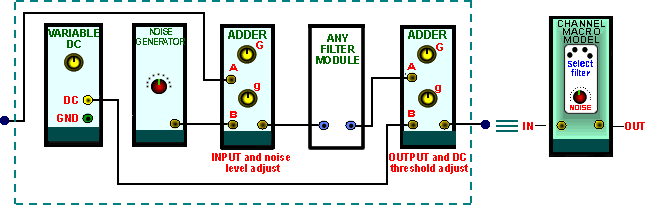 |
| Figure 3: details of the macro CHANNEL MODEL module |
Typically, in a TIMS model, the gain through the channel would be set to unity . This requires that the upper gain control, 'G', of both ADDER modules, be set to unity. Both the BASEBAND CHANNEL FILTER module and the 100 kHz CHANNEL FILTER module have fixed gains of unity. If the TUNEABLE LPF is used, then its adjustable gain must also be set to about unity.
However, in particular instances, these gains may be set otherwise.The noise level is adjusted by both the lower gain control 'g' of the INPUT ADDER and the front panel calibrated attenuator of the NOISE GENERATOR module. Typically the gain would be set to zero [g fully anti-clockwise] until noise is required. Then the general noise level is set by g, and changes of precise magnitude introduced by the calibrated attenuator.
Theory often suggests to us the means of making small improvements to SNR in a particular system. Although small, they can be of value, especially when combined with other small improvements implemented elsewhere. An improvement of 6 dB in received SNR can mean a doubling of the range for reception from a satellite, for example.
You should look now at the Tutorial Questions, as important preparation for the experiment.
These days even the most modest laboratory is equipped with computer controlled apparatus which makes the measurement of a filter response in a few seconds, and provides the output result in great detail. At the very least this is in the form of amplitude, phase, and group delay responses in both soft and hard copy.
It is instructive, however, to make at least one such measurement using what might be called 'first principles'. In this experiment you will make a measurement of the amplitude-versus-frequency response of one of the BASEBAND CHANNEL FILTERS .
A typical measurement arrangement is illustrated in Figure 4 below.
 |
| Figure 4: measurement of filter amplitude response |
In the arrangement of Figure 4:
The audio oscillator provides the input to the filter,
at the TIMS ANALOG REFERENCE LEVEL, and over a frequency range suitable for
the filter being measured.
The BUFFER allows fine adjustment of the signal amplitude into the filter. It
is always convenient to make the measurement with a constant amplitude signal
at the input to the device being measured. The
TIMS AUDIO
OSCILLATOR
output amplitude is reasonably constant as the frequency changes,
but should be monitored in this sort of measurement situation.
The filter can be selected from the three in the module by the front panel switch
(positions #2, #3, and #4). Each has a gain in the passband of around unity.
Remember there is a' straight through , path -switch position # l
The
WIDEBAND TRUE RMS METER
will measure the amplitude of the output voltage
The
FREQUENCY COUNTER
will indicate the frequency of measurement
The OSCILLOSCOPE will monitor the output waveform. With TIMS there is unlikely to be any overloading of the filter if analog signals remain below the TIMS ANALOG REFERENCE LEVEL; but it is always a good idea in a less controlled situation to keep a constant check that the analog system is operating in a linear manner -not to big and not too small an input signal. This is not immediately obvious by looking at the WIDEBAND TRUE RMS METER reading alone (see Tutorial Q2). Note that the oscilloscope is externally triggered from the constant amplitude source of the input signal.
The measuring procedure is:
T1
Decide upon a frequency range, and the approximate
frequency increments to be made over this range. A preliminary sweep is useful.
It could locate the corner frequency, and the frequency increments you choose
near the comer (where the amplitude-frequency change is fastest) could be closer
together.
T2
Set the AUDIO OSCILLATOR frequency to the low
end of the sweep range. Set the filter input voltage to a convenient value using the
BUFFER AMPLIFIER.
A round figure is often
chosen to make subsequent calculations easier -say 1 volt rms. Note that
the input voltage can be read; without the need to change patching leads,
by switching the front panel switch on the BASEBAND CHANNEL FILTERS module to
the straight-through condition -position # 1. Record the chosen
input voltage amplitude.
T3
Switch back to the chosen filter, and record
the output voltage amplitude and the frequency
T4
Tune to the next frequency. Check that the input amplitude has remained constant; adjust, if necessary, with the
BUFFER AMPLIFIER. Record the output voltage amplitude and the measurement frequency.
T5 Repeat the previous Task until the full frequency range has been covered.
The measurements have been recorded. The next step is usually to display them graphically .This you might like to do using your favorite software graphics package. But it is also instructive -at least once in your career -to make a plot by hand, since, instead of some software deciding upon the axis ranges, you will need to make this decision yourself!
Conventional engineering practice is to plot amplitude in decibels on a linear scale, and to use a logarithmic frequency scale. Why ? See Tutorial Question Q1.
A decibel amplitude scale requires that a reference voltage be chosen. This will be your recorded input voltage. Since the response curve is shown as a ratio, there is no way of telling what this voltage was from most response plots, so it is good practice to note it somewhere on the graph.
T6 Make a graph of your results. Choose your scales wisely. Compare with the theoretical response (in Appendix A).
This next part of the experiment will introduce you to some of the problems and techniques of signal-to-noise ratio measurements.
The maximum output amplitude available from the NOISE GENERATOR is about the TIMS ANALOG REFERENCE LEVEL when measured over a wide bandwidth -that is, wide in the TIMS environment, or say about 1 MHz. This means that, as soon as the noise is bandlimited, as it will be in this experiment, the rms value will drop significantly* (To overcame the problem the noise could first be bandlimited, then amplified).
You will measure both
![]() ,
(ie, SNR) and
,
(ie, SNR) and ![]() , and compare
calculations of one from a measurement of the other.
, and compare
calculations of one from a measurement of the other.
The uncalibrated gain control of the ADDER is used for the adjustment of noise level to give a specific SNR. The TIMS NOISE GENERATOR module has a calibrated attenuator which allows the noise level to be changed in small calibrated steps.
Within the test setup you will use the macro CHANNEL MODEL module already defined. It is shown embedded in the test setup in Figure 5 below.
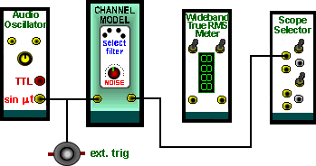 |
| Figure 5: measurement of signal-to-noise ratio |
As in the filter response measurement, the oscilloscope is not essential, but certainly good practice, in an analog environment. It is used to monitor waveforms, as a check that overload is not occurring.
The oscilloscope display will also give you an appreciation of what signals look like with random noise added.
T7
Set up the arrangement of Figure 5 above.
Use the channel model of Figure 3. In this experiment use a
BASEBAND
CHANNEL FILTERS module (select, say, filter #3).
You are now going to set up independent levels of signal
and noise, as recorded by the WIDEBAND TRUE RMS
METER, and then predict
the meter reading when they are present together. After bandlimiting there will
be only a small rms noise voltage available, so this will be set up first.
T8
Reduce to zero the amplitude of the sinusoidal
signal into the channel, using the 'G ' gain control of the
INPUT ADDER.
T9
Set the front panel attenuator of the NOISE GENERATOR to maximum output.
T10 Adjust the gain control 'g' of the INPUT ADDER to maximum. Adjust the 'G' , control of the OUTPUT ADDER for about 1 volt rms. Record the reading. The level of signal into the BASEBAND CHANNEL FILTERS module may exceed the TlMS ANALOG REFERENCE LEVEL, and be close to overloading it -but we need as much noise out as possible. If you suspect overloading, then reduce the noise 2 dB with the attenuator, and check that the expected change is reflected by the rms meter reading. If not, use the INPUT ADDER to reduce the level a little, and check again.
Before commencing the experiment proper have a look at
the noise alone; first wideband, then filtered.
T11
Switch the BASEBAND CHANNEL FILTERS module
to the straight-through connection - switch position #1. Look at the
noise on the oscilloscope.
T12 Switch the BASEBAND CHANNEL FILTERS module to any or all of the lowpass characteristics. Look at the noise on the oscilloscope.
Probably you saw what you expected when the channel was not bandlimiting the noise -an approximation to wideband white noise.
But when the noise was severely bandlimited there is quite a large change. For example:
The amplitude dropped significantly. Knowing the filter bandwidth you could make an estimate of the noise bandwidth before bandlimiting
?
The appearance of the noise in the time domain changed quite significantly. You might like to repeat the last two tasks, using different sweep speeds, and having a closer look at the noise under these two different conditions.
Record your observations. When satisfied:
T13 Reduce to zero the
amplitude of
the noise into the channel by removing its patch cord from the INPUT
ADDER,
thus not disturbing the ADDER adjustment.
T14
Set the AUDIO OSCILLATOR to any convenient
frequency within the passband of the channel. Adjust the gain 'G' of the
INPUT
ADDER until the WIDEBAND TRUE RMS METER reads the same value as it did earlier
for the noise level.
T15
Turn to your note book, and calculate what
the WIDEBAND TRUE RMS METER will read when the noise is reconnected
T16
Replace the noise patch cord into the INPUT ADDER. Record what the meter reads.
T17
Calculate and record the signal-to-noise
ratio in dB.
T18
Measure the signal-plus-noise, then the noise
alone, and calculate the SNR in dB. Compare with the result of the previous
Task.
T19
Increase the signal level, thus changing
the SNR. Measure both
![]() , and
, and
![]() , and predict each from the measurement of the other.
Repeat for different SNR.
, and predict each from the measurement of the other.
Repeat for different SNR.
It is interesting to listen to speech corrupted
by noise. You will be able to obtain a qualitative idea of
various levels of signal-to-noise ratios.
T20
Obtain speech either from TRUNKS or a SPEECH
MODULE. Listen to it using the HEADPHONE AMPLIFIER alone. Switch the in-built
LPF in and out and observe any change of the speech quality. Comment. The filter
has a cut-off of 3 kHz -confirm this by measurement.
T21
Pass the speech through the macro CHANNEL
MODEL module, using the BASEBAND CHANNEL FILTERS module as the band limiter.
Add noise and observe, qualitative/y, the sound of different levels of signal-to-noise
ratio.
T22 What can you say about the intelligibility of the speech when corrupted by noise ? If you are using bandlimited speech, but wideband noise, you can make observations about the effect upon intelligibility of restricting the noise to the same bandwidth as the speech. Do this, and report your conclusions.
T23 How easy is it to measure the signal power, when
it is speech ? Comment. Remember: it is easy to introduce a precise
change
to the SNR (how ?), but with speech the measurement
of absolute level of SNR is not as straightforward as with a sinusoidal
message.
How might you have measured, or estimated, or at least demonstrated the existence of, a time delay through any of the filters ?
hint: try using the SEQUENCE GENERATOR on a short sequence.
Q1 When plotting filter amplitude responses it is customary to use decibel scales for the amplitude, versus a logarithmic .frequency scale. Discuss some of the advantages of this form of presentation over alternatives.
Q2
An analog channel is overloaded with
a single sinewave test signal. Is this always immediately obvious if examined
with an oscilloscope ?
Is it obvious with.
A single measurement using a voltmeter ?
Two or more measurements with a voltmeter ?
Explain you answers to (a) and (b).
Q3
Suppose an rms voltmeter reads
1 volt
at the output of a noisy channel when the signal is removed from the
input. What would it read if the bandwidth was halved ? State any assumptions which were necessary for this answer.
Q4
A sinusoidal waveform has
a peak-to-peak amplitude of
5 volts. What is its rms value ?
Q5
What would an rms meter read
if connected
to a square wave:
Alternating between O and 5 volt ?
Alternating between ±5 volt ?
Q6
The measuring instrument used in this experiment
was an rms volt meter. Could you derive a conversion factor so
that the instrument could be used as a direct reading (relative) power meter ?
Q7
Suppose a meter is reading 1 volt rms on a pure tone. Wideband noise is now
added until the meter reading increases by 10%.
What would be the signal-to-noise ratio in dB?
What would the rms volt meter read on noise alone?
This answer is meant to measuring small changes to signal-to-noise ratios is difficult unless the signal-to-noise ratio is already small. Do you agree? How small?* (This is a value judgment, so answers may vary. But it is not 40 dB, for example. Do you agree?)
Q8 Wideband white noise is
passed through a lowpass filter to a meter. If the filter bandwidth is decreased
by one half, what would be the change of the reading of the meter if:
It responds to power - answer in dB
It is a true rms volt meter - give the percent change
Q9
Explain how you might measure, or at least demonstrate the existence of, a time
delay through any of the filters?
|
|
Go to ECE489 Experiment | 1 | 2 | 3 | 4 | 5 | 6 | 7 | 8 | 10 | 11 | 12 | 13 | 14 | ECE Lab home |
|