Go to  ECE489  Experiment  |   1   |    2   |   3   |   4   |   5   |   6   |   7   |   8   |   9   |   10  |   11   |   12   |  13  |  14   |      ECE Lab home

 ECE 489 Communications Systems Laboratory

Experiment 1: Distortion Analysis

Distortion Analysis - A Tutorial

The object of this experiment is to become familiar with the concept of distortion and to get some practical experience in the performance of distortion measurements. Before proceeding, a short review will be undertaken.

A distortionless device is one that produces an output v(t) which is a scaled and delayed version of an input x(t). We could summarize the relationship by

where k is the scale factor and td is the delay of the device.

You might argue that a telephone conversation that is scaled in amplitude, provided it is audible and not earshattering, is equally as comprehensible as the unscaled version. Within reasonable bounds, a short delay in the reception of a message will not change anything. After all, we tolerate delays of more than 15 milliseconds in coast to coast conversations without taking notice.

If a device is not linear then it causes distortion. In (4.1), we will leave the delay td out of the discussion without losing any generality. So a distortionless device should obey the linear relation

         Any device in which the output is not linearly related to the input causes distortion. For example

will cause distortion.    The easiest way of quantifying distortion is to use a sinusoidal test signal

If we use

in ( 4.2) then we get an output

which is a scaled replica of the sinusoidal input.

    If, on the other hand, we use (4.4) in (4.3) then we get the output

   To the above we apply some trigonometric identities to obtain

which indicates that at the output we have signals that we did not have at the input. The excessive signals represent distortion.

For a periodic signal, which can always be written as a Fourier expansion, the distortion is defined as the ratio of the rms value of all components other than the fundamental to the rms value of the fundamental. The distortion D, of the signal in ( 4.7), is

(4.8)

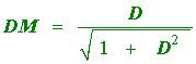
The analyzer at our disposal does not measure the above quantity, but rather

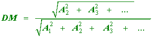(4.9)

It uses as a definition of distortion the ratio of the rms value of all components other than the fundamental to the rms value of the entire signal.

    It is very easily verified that the measured and defined distortion are related by

    and

For small values of distortion, D and DM are very close to each other. For values of measured distortion greater than 0.1 it is worthwhile to use (4.10) to find the true distortion, particularly if greater accuracy is desired.

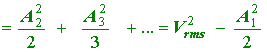
When dealing with a periodic waveshape of known form we may use a short- cut in calculating the distortion. We base this method on the idea that the mean square value of the waveform is the sum of the mean square values of all of its harmonics. Thus

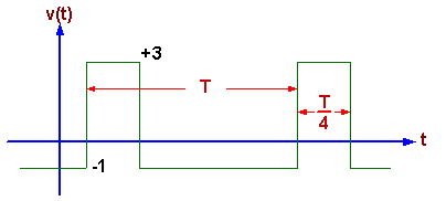
Figure 4.1: A 25% duty cycle rectangular wave.

where we used V_rms to represent the rms value of the signal in ( 4.7 )

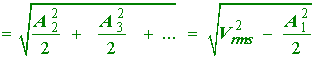
We rearrange the last equation into

Taking the square root of both sides we obtain

The left hand side of the above equation is the rms value of all the distortion harmonics. This value divided by V_rms is the reading that the audio analyzer should display. (4.14)

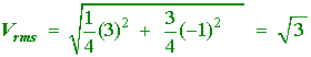
These ideas will be illustrated with an example. Consider the 25% duty cycle rectangular wave shown in figure 4.1. We wish find the expected reading of the analyzer in terms of DM .

For this example the rms value can be calculated by simply looking at the wave. The result is

For a rectangular pulse train with pulse height V, period T and duty cycle  t / T  we find that the Fourier coefficients are given by

In our example V = 4 and  t / T = 1/4. Therefore the above reduces to

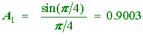
and we only need to know A₁, which is

According to (4.14)

rms value of distortion

(4.19)

The measured value of DM should therefore be close to

Now we know what we could expect for a distortion measurement of the rectangular wave of figure 4.1.

Top    |    ECE489 Index

In your report answers the questions below.

1.    What is the relationship of the coefficients of ( 4.7 ) to those in ( 4.6 ) ?

2.     Derive  (4.11)  from  ( 4.10 )  and vice versa.

 

THE EXPERIMENT

The required equipment is an HP 8903B audio analyzer and instruction manual, which are available in the stockroom.

1.     Measure the distortion of the internal source of the analyzer. (This is just a check of the instrument.)

2.     Measure the distortion of the sine wave output of the Wavetek generator at several frequencies between 100 Hz and 10 kHz.

3.     Repeat for a triangle wave and a square wave at a frequency of 1 kHz. In your report, compare the measured valves and what you would expect from theoretical considerations.

4.     Build a one stage transistor or OP-AMP amplifier with a voltage gain of » 40. Increase the input signal so the output signal is barely showing signs of distortion. Measure the distortion using the distortion analyzer so that you can answer the question which follows.

What is the approximate value of the minimum distortion you are able to observe visually on the oscilloscope ?

Go to  ECE489  Experiment  |   1   |    2   |   3   |   4   |   5   |   6   |   7   |   8   |   9   |   10  |   11   |   12   |  13   |  14   |       ECE Lab home